Track OTs

%pylab inline

import pandas as pd
import glob
import os

import numpy as np
import pandas as pd

import trackpy as tp
from copy import deepcopy
import pyproj

import xarray as xr
import cartopy.crs as ccrs

dem_files = sorted(glob.glob('/data/accp/a/snesbitt/relampago/srtm/*.tif'))

ds_list = []
for file in dem_files:
    ds_list.append(xr.open_rasterio(file).isel(band=0))
import scipy
from shapely import wkt
import geopandas as gpd

ota_bins = np.arange(0, 225, 25)
otd_bins = np.arange(0, 4, .2)
dur_bins = np.arange(3, 16, 1)

Populating the interactive namespace from numpy and matplotlib

10 November Case

df = pd.concat([pd.read_csv(f) for f in sorted(glob.glob('ot_output/20181110/20181110*'))], ignore_index = True).drop(columns='Unnamed: 0')

df['geometry'] = df['geometry'].apply(wkt.loads)
geo_df = gpd.GeoDataFrame(df, geometry='geometry')

df = geo_df

df['ot_depth'] = df['cloudtop_height'] - df['tropopause_height']

df['diff'] = pd.to_datetime(df['time']) - pd.datetime(2018,11,1)
df['frame'] = df['diff'].dt.days*86400+df['diff'].dt.seconds
df['frame'] = df['frame'] - df['frame'].min()

/data/keeling/a/mgrover4/a/miniconda3/envs/xesmf_env/lib/python3.7/site-packages/ipykernel_launcher.py:1: FutureWarning: The pandas.datetime class is deprecated and will be removed from pandas in a future version. Import from datetime module instead.
  """Entry point for launching an IPython kernel.

df['time'] = pd.to_datetime(df.time)

df['hour'] = df.time.dt.hour
df['minute'] = df.time.dt.minute

df = df[df.prob > .8]

good_ind = df['lat'].apply(lambda x: pd.to_numeric(x, errors='coerce')).index

df = df[df.index == good_ind]

df_track = deepcopy(df)
#df_track.rename(columns={'lon':'x', 'lat':'y'}, inplace=True)
#df_track['z'] = 0
df_track['states'] = 0
df_track['label'] = 0

radius=6371228.

globe = ccrs.Globe(ellipse=None, semimajor_axis=radius, 
                   semiminor_axis=radius)

projection=ccrs.LambertAzimuthalEqualArea(central_latitude=-32.,
                                          central_longitude=-62.,globe=globe)

prj=pyproj.Proj(projection.proj4_init)

df_track['x'], df_track['y'] = prj(df_track['lon'].values, df_track['lat'].values)


df_track.to_csv('test.csv')

v_max=60.
stubs=2
order=1
extrapolate=1
memory=1
adaptive_stop=0.01
adaptive_step=0.99
subnetwork_size=100
method_linking= 'predict'
cell_number_start=1
dt = 60.
dxy = 2000.

search_range=dt*v_max

features_linking=deepcopy(df_track)

pred = tp.predict.NearestVelocityPredict(span=1)
trajectories_unfiltered = pred.link_df(features_linking, search_range=search_range, memory=memory,
                                 pos_columns=['x','y'],
                                 t_column='frame',
                                 neighbor_strategy='KDTree', link_strategy='auto',
                                 adaptive_step=adaptive_step,adaptive_stop=adaptive_stop
#                                 copy_features=False, diagnostics=False,
#                                 hash_size=None, box_size=None, verify_integrity=True,
#                                 retain_index=False
                                 )

trajectories_unfiltered['cell']=None
for i_particle,particle in enumerate(pd.Series.unique(trajectories_unfiltered['particle'])):
    cell=int(i_particle+cell_number_start)
    trajectories_unfiltered.loc[trajectories_unfiltered['particle']==particle,'cell']=cell
trajectories_unfiltered.drop(columns=['particle'],inplace=True)

trajectories_bycell=trajectories_unfiltered.groupby('cell')

num_stubs = 0

for cell,trajectories_cell in trajectories_bycell:
#    logging.debug("cell: "+str(cell))
#    logging.debug("feature: "+str(trajectories_cell['feature'].values))
#    logging.debug("trajectories_cell.shape[0]: "+ str(trajectories_cell.shape[0]))


    if trajectories_cell.shape[0] < stubs:
#        print("cell" + str(cell)+ "  is a stub ("+str(trajectories_cell.shape[0])+ "), setting cell number to Nan..")
        trajectories_unfiltered.loc[trajectories_unfiltered['cell']==cell,'cell']=np.nan
        num_stubs = num_stubs + 1

print('found this many stubs: {}'.format(num_stubs))

Frame 27841: 5 trajectories present.
found this many stubs: 116

trajectories_filtered=trajectories_unfiltered.dropna(subset=['area_polygon', 'ot_depth'])

cells_grouped = trajectories_filtered.groupby('cell')

trajectories_filtered.time = pd.to_datetime(trajectories_filtered.time)

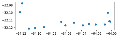
supercell = trajectories_filtered[trajectories_filtered.cell == 93]

supercell.centroid.plot()

<AxesSubplot:>

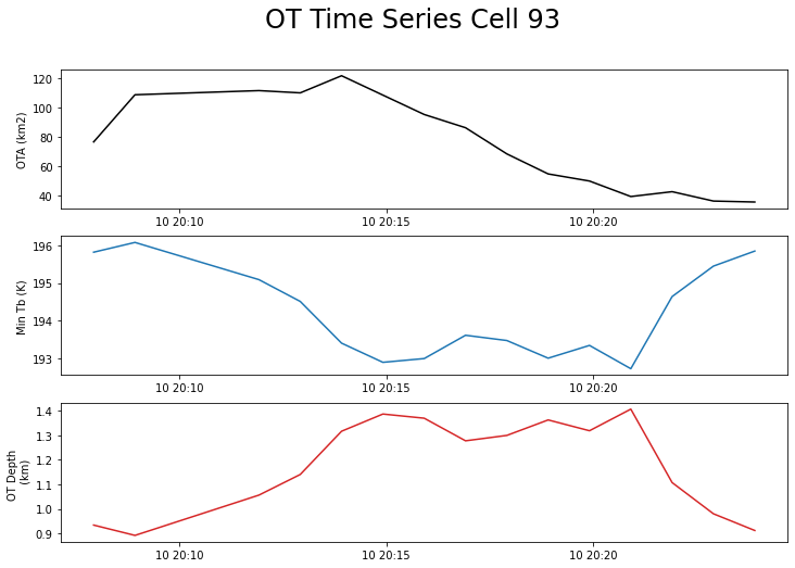
ota = supercell.area_polygon.values
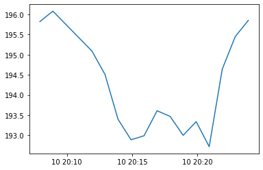
mintb = supercell.mintb.values
hgt = supercell.ot_depth.values

times = pd.to_datetime(supercell.time)

plt.plot(times, mintb)

[<matplotlib.lines.Line2D at 0x2b96c764bc88>]

plt.plot(times, np.gradient(hgt)*16.6667)

---------------------------------------------------------------------------
NameError                                 Traceback (most recent call last)
<ipython-input-114-c1215faefe8c> in <module>
----> 1 plt.plot(times, np.gradient(hgt)*16.6667)

NameError: name 'times' is not defined

plt.figure(figsize=(12, 8))

ax = plt.subplot(311)
ax.plot(times, ota, color='black')
plt.ylabel('OTA (km2)')

ax = plt.subplot(312)
ax.plot(times, mintb, color='tab:blue')
plt.ylabel('Min Tb (K)')

ax = plt.subplot(313)
ax.plot(times, hgt, color='tab:red')
plt.ylabel('OT Depth \n (km)')

plt.suptitle('OT Time Series Cell 93', fontsize=24)

plt.savefig('cell93_timeseries.png', dpi=300)

duration = cells_grouped.count().area_polygon.values
max_depth = cells_grouped.max().ot_depth.values
mean_depth = cells_grouped.mean().ot_depth.values
max_otarea = cells_grouped.max().area_polygon.values
mean_otarea = cells_grouped.mean().area_polygon.values

df_max = cells_grouped.max()
df_max['duration']= cells_grouped.count().area_polygon

#cells_grouped.count().area_polygon

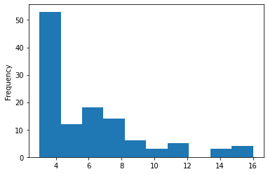
df_max[df_max.duration >2].duration.plot.hist()

<AxesSubplot:ylabel='Frequency'>

def plot_regression(x, y, xlabel='OT Duration (minutes)', ylabel='OT Area ($km^{2}$)', plot_label = 'OT Duration 10 November 2018 \n 1500 - 2359 UTC (Count = 179)'):
    slope, intercept, r, p, stderr = scipy.stats.linregress(x, y)
    
    line = f'Regression line: y={intercept:.2f}+{slope:.2f}x, r={r:.2f}'
    
    plt.figure(figsize=(10,8))
    ax = plt.subplot(111)
    ax.scatter(x, y)
    ax.plot(np.array(x), intercept + slope * np.array(x), label=line, color='black')

    plt.ylabel(ylabel, fontsize=12)
    plt.xlabel(xlabel, fontsize=12)

    plt.legend(loc='upper right', fontsize=12)

    plt.title(plot_label, fontsize=16)

ota_bins = np.arange(0, 225, 25)
otd_bins = np.arange(0, 4, .2)
dur_bins = np.arange(3, 16, 1)

fig = plt.figure(figsize=(12,8))
plt.hist(df_max.area_polygon, bins=ota_bins)

plt.title('OTA Distribution \n 10 November 2018 1500 - 0000 UTC', fontsize=24)

plt.xlabel('OTA ($km^2$)', fontsize=16)
plt.ylabel('Frequency', fontsize=16)

Text(0, 0.5, 'Frequency')

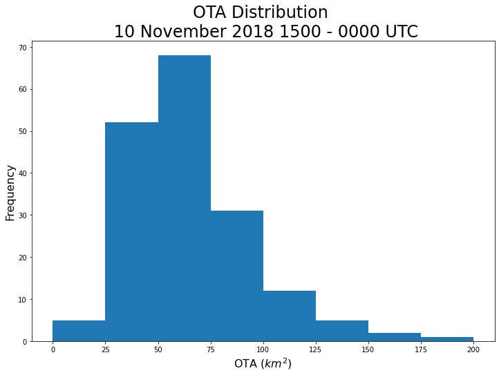
fig = plt.figure(figsize=(12,8))
plt.hist(df_max.ot_depth, bins=otd_bins)

plt.title('OT Depth Distribution \n 10 November 2018 1500 - 0000 UTC', fontsize=24)

plt.xlabel('OT Depth (km)', fontsize=16)
plt.ylabel('Frequency', fontsize=16)

Text(0, 0.5, 'Frequency')

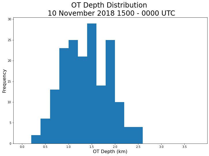
fig = plt.figure(figsize=(12,8))
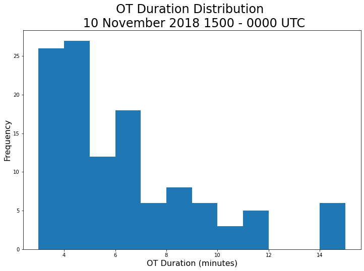
plt.hist(df_max.duration, bins=dur_bins)

plt.title('OT Duration Distribution \n 10 November 2018 1500 - 0000 UTC', fontsize=24)

plt.xlabel('OT Duration (minutes)', fontsize=16)
plt.ylabel('Frequency', fontsize=16)

Text(0, 0.5, 'Frequency')

plot_regression(df_max.duration, df_max.area_polygon)

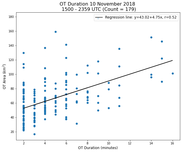
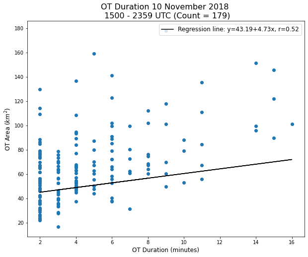
slope, intercept, r, p, stderr = scipy.stats.linregress(duration, max_otarea)

line = f'Regression line: y={intercept:.2f}+{slope:.2f}x, r={r:.2f}'
line

'Regression line: y=43.19+4.73x, r=0.52'

slope, intercept, r, p, stderr = scipy.stats.linregress(duration, mean_otarea)
r

0.35167524403770134

len(duration)

177

plt.figure(figsize=(10,8))
ax = plt.subplot(111)
ax.scatter(duration, max_otarea)
ax.plot(np.array(duration), intercept + slope * np.array(duration), label=line, color='black')

plt.ylabel('OT Area ($km^{2}$)', fontsize=12)
plt.xlabel('OT Duration (minutes)', fontsize=12)

plt.legend(loc='upper right', fontsize=12)

plt.title('OT Duration 10 November 2018 \n 1500 - 2359 UTC (Count = 179)', fontsize=16)

Text(0.5, 1.0, 'OT Duration 10 November 2018 \n 1500 - 2359 UTC (Count = 179)')

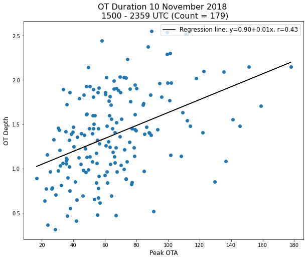
plot_regression(max_otarea, max_depth, xlabel='Peak OTA', ylabel='OT Depth')

import seaborn as sns
sns.set()
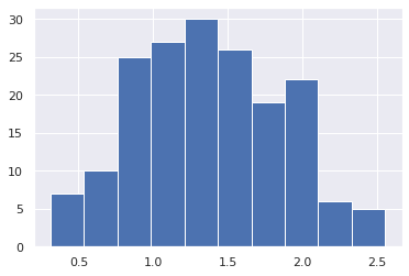
plt.hist(max_depth)

(array([ 7., 10., 25., 27., 30., 26., 19., 22.,  6.,  5.]),
 array([0.31200027, 0.5361002 , 0.76020012, 0.98430004, 1.20839996,
        1.43249989, 1.65659981, 1.88069973, 2.10479965, 2.32889957,
        2.5529995 ]),
 <BarContainer object of 10 artists>)

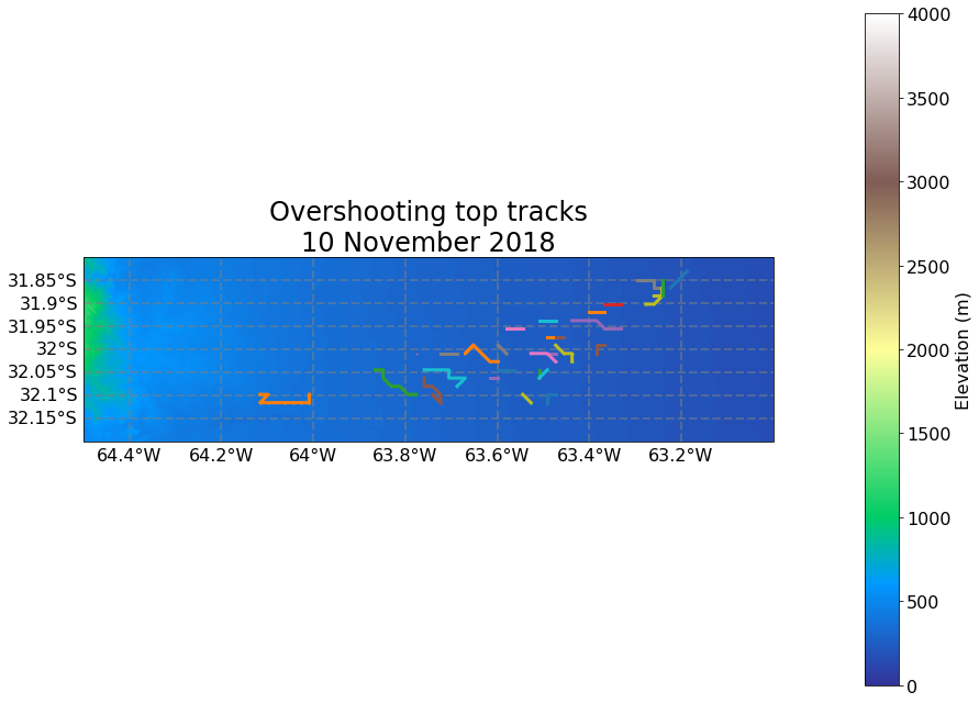
llcrnr=[-32.2, -64.5]
urcrnr=[-31.8, -63.]

# Set extent of maps created in the following cells:
axis_extent=[llcrnr[1],urcrnr[1],llcrnr[0],urcrnr[0]]    

# Plot map with all individual tracks:
import cartopy.crs as ccrs
fig_map,ax_map=plt.subplots(figsize=(15,15),subplot_kw={'projection': ccrs.PlateCarree()})

ax_map.coastlines()

ax_map.set_extent(axis_extent)

for ds in ds_list:
#    cm = ax.contourf(ds.x.values[::5], ds.y.values[::5], ds.values[::5,::5], levs, cmap='terrain', transform=ccrs.PlateCarree())
    cm = ax_map.imshow(ds.values, extent =[ds.x.min(),ds.x.max(),ds.y.min(),ds.y.max()], transform=ccrs.PlateCarree(), vmin=0, vmax=4000, cmap='terrain')

gl = ax_map.gridlines(crs=ccrs.PlateCarree(), draw_labels=True,
                  linewidth=2, color='gray', alpha=0.5, linestyle='--')

gl.top_labels = False
gl.left_labels= True
gl.right_labels = False
gl.xlabel_style = {'size': 16, 'color': 'k'}
gl.ylabel_style = {'size': 16, 'color': 'k'}

for name, group in cells_grouped:
#    print(group.x,group.y)
    plt.plot(group.lon,group.lat,"-o",markersize=1, linewidth=3)

cb = plt.colorbar(cm,label='Elevation (m)',shrink=0.75, pad=0.1)
cb.ax.tick_params(labelsize=16)
cb.set_label('Elevation (m)', fontsize=16)

ax_map.set_title('Overshooting top tracks\n10 November 2018', fontsize=24)
plt.savefig('ot_10_nov.png', dpi=300)

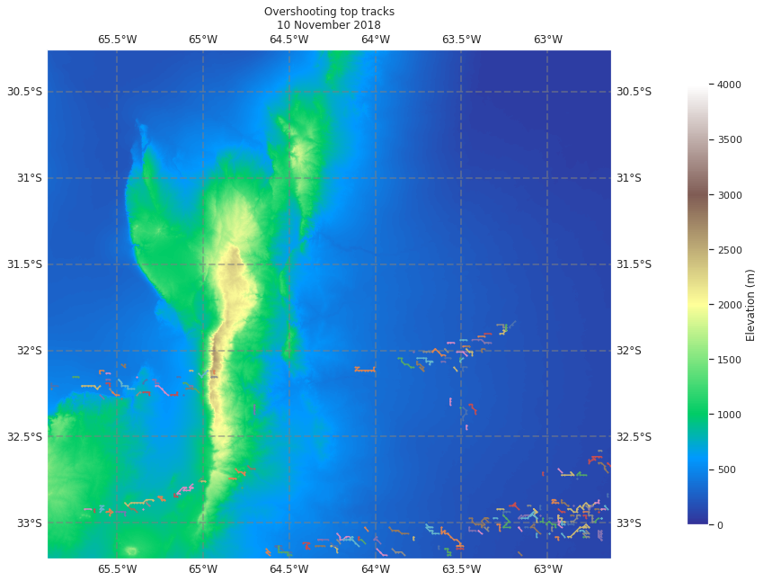
llcrnr=[-33.206342, -65.906586]
urcrnr=[-30.255825, -62.630553]

# Set extent of maps created in the following cells:
axis_extent=[llcrnr[1],urcrnr[1],llcrnr[0],urcrnr[0]]    

# Plot map with all individual tracks:
import cartopy.crs as ccrs
fig_map,ax_map=plt.subplots(figsize=(15,15),subplot_kw={'projection': ccrs.PlateCarree()})

ax_map.coastlines()

ax_map.set_extent(axis_extent)

for ds in ds_list:
#    cm = ax.contourf(ds.x.values[::5], ds.y.values[::5], ds.values[::5,::5], levs, cmap='terrain', transform=ccrs.PlateCarree())
    cm = ax_map.imshow(ds.values, extent =[ds.x.min(),ds.x.max(),ds.y.min(),ds.y.max()], transform=ccrs.PlateCarree(), vmin=0, vmax=4000, cmap='terrain')

gl = ax_map.gridlines(crs=ccrs.PlateCarree(), draw_labels=True,
                  linewidth=2, color='gray', alpha=0.5, linestyle='--')

for name, group in cells_grouped:
#    print(group.x,group.y)
    plt.plot(group.lon,group.lat,"-o",markersize=1)

plt.colorbar(cm,label='Elevation (m)',shrink=0.6, pad=0.1)

ax_map.set_title('Overshooting top tracks\n10 November 2018')

Text(0.5, 1.0, 'Overshooting top tracks\n10 November 2018')

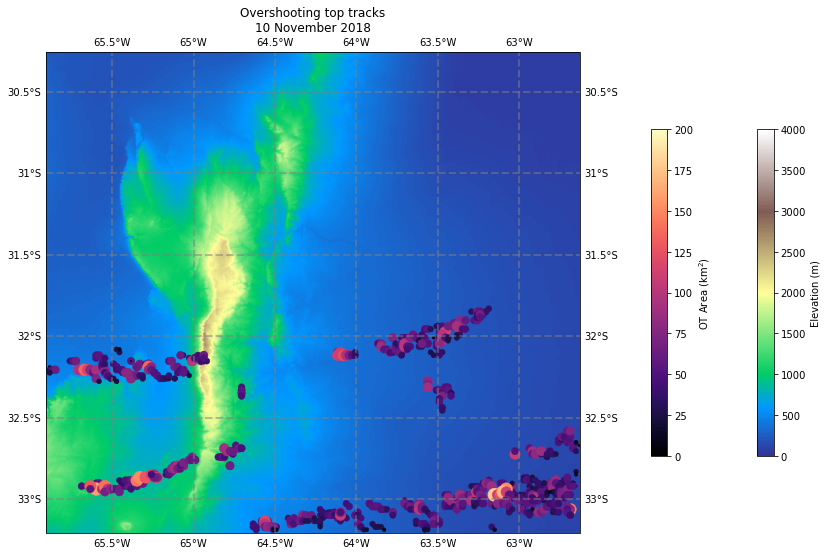
llcrnr=[-33.206342, -65.906586]
urcrnr=[-30.255825, -62.630553]

# Set extent of maps created in the following cells:
axis_extent=[llcrnr[1],urcrnr[1],llcrnr[0],urcrnr[0]]    

# Plot map with all individual tracks:
import cartopy.crs as ccrs
fig_map,ax_map=plt.subplots(figsize=(15,15),subplot_kw={'projection': ccrs.PlateCarree()})

ax_map.coastlines()

ax_map.set_extent(axis_extent)

for ds in ds_list:
#    cm = ax.contourf(ds.x.values[::5], ds.y.values[::5], ds.values[::5,::5], levs, cmap='terrain', transform=ccrs.PlateCarree())
    cm = ax_map.imshow(ds.values, extent =[ds.x.min(),ds.x.max(),ds.y.min(),ds.y.max()], transform=ccrs.PlateCarree(), vmin=0, vmax=4000, cmap='terrain')

gl = ax_map.gridlines(crs=ccrs.PlateCarree(), draw_labels=True,
                  linewidth=2, color='gray', alpha=0.5, linestyle='--')

for name, group in cells_grouped:
#    print(group.x,group.y)
    cm2 = plt.scatter(group.lon,group.lat,c=group.area_polygon,vmin=0.,vmax=200.,s=group.area_polygon,
                     facecolors='none',cmap='magma',linewidth=0.5)

plt.colorbar(cm,label='Elevation (m)',shrink=0.4, pad=0.0)
plt.colorbar(cm2,label='OT Area (km$^2$)',shrink=0.4, pad=0.1)



ax_map.set_title('Overshooting top tracks\n10 November 2018')

Text(0.5, 1.0, 'Overshooting top tracks\n10 November 2018')

---

12 November Case

df = pd.concat([pd.read_csv(f) for f in sorted(glob.glob('ot_output/20181112/20181112*'))], ignore_index = True).drop(columns='Unnamed: 0')

df['geometry'] = df['geometry'].apply(wkt.loads)
geo_df = gpd.GeoDataFrame(df, geometry='geometry')

df = geo_df

df['diff'] = pd.to_datetime(df['time']) - pd.datetime(2018,11,1)
df['frame'] = df['diff'].dt.days*86400+df['diff'].dt.seconds
df['frame'] = df['frame'] - df['frame'].min()
df['ot_depth'] = df['cloudtop_height'] - df['tropopause_height']

df = df[df.ot_depth > 0]

/data/keeling/a/mgrover4/a/miniconda3/envs/xesmf_env/lib/python3.7/site-packages/ipykernel_launcher.py:6: FutureWarning: The pandas.datetime class is deprecated and will be removed from pandas in a future version. Import from datetime module instead.
  

df = df[df.prob > .7]

df_track = deepcopy(df)
#df_track.rename(columns={'lon':'x', 'lat':'y'}, inplace=True)
#df_track['z'] = 0
df_track['states'] = 0
df_track['label'] = 0

radius=6371228.

globe = ccrs.Globe(ellipse=None, semimajor_axis=radius, 
                   semiminor_axis=radius)

projection=ccrs.LambertAzimuthalEqualArea(central_latitude=-32.,
                                          central_longitude=-62.,globe=globe)

prj=pyproj.Proj(projection.proj4_init)

df_track['x'], df_track['y'] = prj(df_track['lon'].values, df_track['lat'].values)


df_track.to_csv('test.csv')

v_max=60.
stubs=2
order=1
extrapolate=1
memory=1
adaptive_stop=0.01
adaptive_step=0.99
subnetwork_size=100
method_linking= 'predict'
cell_number_start=1
dt = 60.
dxy = 2000.

search_range=dt*v_max

features_linking=deepcopy(df_track)

pred = tp.predict.NearestVelocityPredict(span=1)
trajectories_unfiltered = pred.link_df(features_linking, search_range=search_range, memory=memory,
                                 pos_columns=['x','y'],
                                 t_column='frame',
                                 neighbor_strategy='KDTree', link_strategy='auto',
                                 adaptive_step=adaptive_step,adaptive_stop=adaptive_stop
#                                 copy_features=False, diagnostics=False,
#                                 hash_size=None, box_size=None, verify_integrity=True,
#                                 retain_index=False
                                 )

trajectories_unfiltered['cell']=None
for i_particle,particle in enumerate(pd.Series.unique(trajectories_unfiltered['particle'])):
    cell=int(i_particle+cell_number_start)
    trajectories_unfiltered.loc[trajectories_unfiltered['particle']==particle,'cell']=cell
trajectories_unfiltered.drop(columns=['particle'],inplace=True)

trajectories_bycell=trajectories_unfiltered.groupby('cell')

num_stubs = 0

for cell,trajectories_cell in trajectories_bycell:
#    logging.debug("cell: "+str(cell))
#    logging.debug("feature: "+str(trajectories_cell['feature'].values))
#    logging.debug("trajectories_cell.shape[0]: "+ str(trajectories_cell.shape[0]))


    if trajectories_cell.shape[0] < stubs:
#        print("cell" + str(cell)+ "  is a stub ("+str(trajectories_cell.shape[0])+ "), setting cell number to Nan..")
        trajectories_unfiltered.loc[trajectories_unfiltered['cell']==cell,'cell']=np.nan
        num_stubs = num_stubs + 1

print('found this many stubs: {}'.format(num_stubs))

trajectories_filtered=trajectories_unfiltered.dropna()

Frame 15720: 1 trajectories present.
found this many stubs: 142

len(trajectories_filtered)

346

cells_grouped = trajectories_filtered.groupby('cell')
df_max = cells_grouped.max()
df_max['duration']= cells_grouped.count().area_polygon

df_max = df_max[df_max.duration > 2]

duration = cells_grouped.count().area_polygon.values
max_depth = cells_grouped.max().ot_depth.values
mean_depth = cells_grouped.mean().ot_depth.values
max_otarea = cells_grouped.max().area_polygon.values
mean_otarea = cells_grouped.mean().area_polygon.values

slope, intercept, r, p, stderr = scipy.stats.linregress(df_max.duration, df_max.area_polygon)

line = f'Regression line: y={intercept:.2f}+{slope:.2f}x, r={r:.2f}'

plt.figure(figsize=(10,8))
ax = plt.subplot(111)
ax.scatter(duration, max_otarea)
ax.plot(np.array(duration), intercept + slope * np.array(duration), label=line, color='black')

plt.ylabel('OT Area ($km^{2}$)', fontsize=12)
plt.xlabel('OT Duration (minutes)', fontsize=12)

plt.legend(loc='upper right', fontsize=12)

plt.title('OT Duration 12 November 2018 \n 0000 - 0600 UTC (Count = 563)', fontsize=16)

Text(0.5, 1.0, 'OT Duration 12 November 2018 \n 0000 - 0600 UTC (Count = 563)')

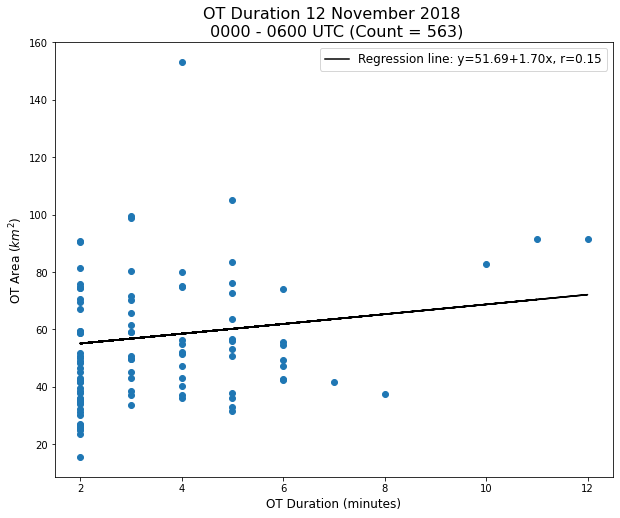
fig = plt.figure(figsize=(12,8))
plt.hist(df_max.area_polygon, bins=ota_bins)

plt.title('OTA Distribution \n 12 November 2018 0130 - 0553 UTC', fontsize=24)

plt.xlabel('OTA ($km^2$)', fontsize=16)
plt.ylabel('Frequency', fontsize=16)

Text(0, 0.5, 'Frequency')

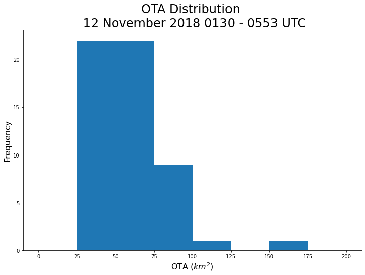
fig = plt.figure(figsize=(12,8))
plt.hist(df_max.ot_depth, bins=otd_bins)

plt.title('OT Depth Distribution \n 12 November 2018 0130 - 0553 UTC', fontsize=24)

plt.xlabel('OT Depth (km)', fontsize=16)
plt.ylabel('Frequency', fontsize=16)

Text(0, 0.5, 'Frequency')

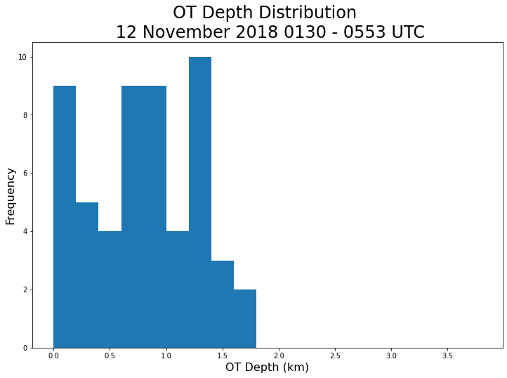
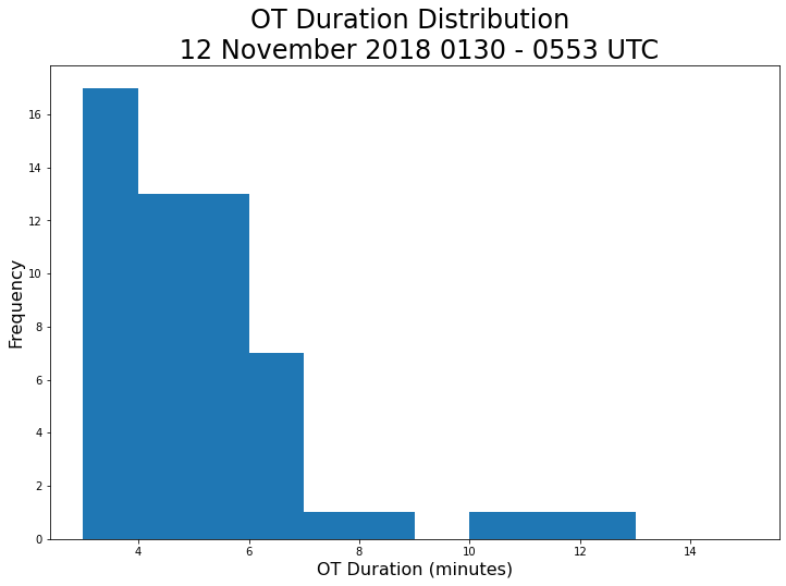
fig = plt.figure(figsize=(12,8))
plt.hist(df_max.duration, bins=dur_bins)

plt.title('OT Duration Distribution \n 12 November 2018 0130 - 0553 UTC', fontsize=24)

plt.xlabel('OT Duration (minutes)', fontsize=16)
plt.ylabel('Frequency', fontsize=16)

Text(0, 0.5, 'Frequency')

df_track['Time'] = pd.to_datetime(df_track.time)

from datetime import datetime

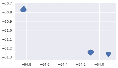
df = df_track[(df_track['Time'] > datetime(2018, 11, 12, 2, 30))][(df_track.Time < datetime(2018, 11, 12, 2, 34))]

/data/keeling/a/mgrover4/a/miniconda3/envs/xesmf_env/lib/python3.7/site-packages/geopandas/geodataframe.py:546: UserWarning: Boolean Series key will be reindexed to match DataFrame index.
  result = super(GeoDataFrame, self).__getitem__(key)

df.columns

Index(['area_polygon', 'cloudtop_height', 'e_radial', 'e_radial_del2', 'e_tb',
       'geometry', 'lat', 'lat_corr', 'lon', 'lon_corr', 'mintb', 'n_radial',
       'n_radial_del2', 'n_tb', 'ne_radial', 'ne_radial_del2', 'ne_tb',
       'nw_radial', 'nw_radial_del2', 'nw_tb', 'otid', 'prob', 's_radial',
       's_radial_del2', 's_tb', 'se_radial', 'se_radial_del2', 'se_tb',
       'sw_radial', 'sw_radial_del2', 'sw_tb', 'time', 'tropopause_height',
       'tropopause_pressure', 'tropopause_temperature', 'w_radial',
       'w_radial_del2', 'w_tb', 'diff', 'frame', 'states', 'label', 'x', 'y',
       'Time'],
      dtype='object')

df[(df.lat > -31.4) & (df.lon < -63.8)].plot()

<AxesSubplot:>

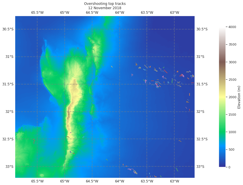
llcrnr=[-33.206342, -65.906586]
urcrnr=[-30.255825, -62.630553]

# Set extent of maps created in the following cells:
axis_extent=[llcrnr[1],urcrnr[1],llcrnr[0],urcrnr[0]]    

# Plot map with all individual tracks:
import cartopy.crs as ccrs
fig_map,ax_map=plt.subplots(figsize=(15,15),subplot_kw={'projection': ccrs.PlateCarree()})

ax_map.coastlines()

ax_map.set_extent(axis_extent)

for ds in ds_list:
#    cm = ax.contourf(ds.x.values[::5], ds.y.values[::5], ds.values[::5,::5], levs, cmap='terrain', transform=ccrs.PlateCarree())
    cm = ax_map.imshow(ds.values, extent =[ds.x.min(),ds.x.max(),ds.y.min(),ds.y.max()], transform=ccrs.PlateCarree(), vmin=0, vmax=4000, cmap='terrain')

gl = ax_map.gridlines(crs=ccrs.PlateCarree(), draw_labels=True,
                  linewidth=2, color='gray', alpha=0.5, linestyle='--')

for name, group in cells_grouped:
#    print(group.x,group.y)
    plt.plot(group.lon,group.lat,"-o",markersize=1)

plt.colorbar(cm,label='Elevation (m)',shrink=0.6, pad=0.1)

ax_map.set_title('Overshooting top tracks\n12 November 2018')

Text(0.5, 1.0, 'Overshooting top tracks\n12 November 2018')

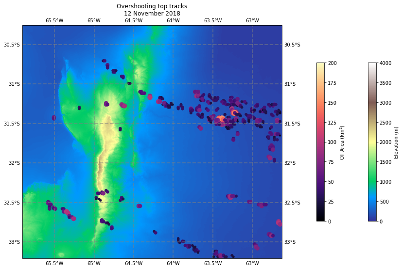
llcrnr=[-33.206342, -65.906586]
urcrnr=[-30.255825, -62.630553]

# Set extent of maps created in the following cells:
axis_extent=[llcrnr[1],urcrnr[1],llcrnr[0],urcrnr[0]]    

# Plot map with all individual tracks:
import cartopy.crs as ccrs
fig_map,ax_map=plt.subplots(figsize=(15,15),subplot_kw={'projection': ccrs.PlateCarree()})

ax_map.coastlines()

ax_map.set_extent(axis_extent)

for ds in ds_list:
#    cm = ax.contourf(ds.x.values[::5], ds.y.values[::5], ds.values[::5,::5], levs, cmap='terrain', transform=ccrs.PlateCarree())
    cm = ax_map.imshow(ds.values, extent =[ds.x.min(),ds.x.max(),ds.y.min(),ds.y.max()], transform=ccrs.PlateCarree(), vmin=0, vmax=4000, cmap='terrain')

gl = ax_map.gridlines(crs=ccrs.PlateCarree(), draw_labels=True,
                  linewidth=2, color='gray', alpha=0.5, linestyle='--')

for name, group in cells_grouped:
#    print(group.x,group.y)
    cm2 = plt.scatter(group.lon,group.lat,c=group.area_polygon,vmin=0.,vmax=200.,s=group.area_polygon,
                     facecolors='none',cmap='magma',linewidth=0.5)

plt.colorbar(cm,label='Elevation (m)',shrink=0.4, pad=0.0)
plt.colorbar(cm2,label='OT Area (km$^2$)',shrink=0.4, pad=0.1)



ax_map.set_title('Overshooting top tracks\n12 November 2018')

Text(0.5, 1.0, 'Overshooting top tracks\n12 November 2018')

14 December Case

df = pd.concat([pd.read_csv(f) for f in sorted(glob.glob('ot_output/20181214/20181214*'))], ignore_index = True).drop(columns='Unnamed: 0')

df['geometry'] = df['geometry'].apply(wkt.loads)
geo_df = gpd.GeoDataFrame(df, geometry='geometry')

df['ot_depth'] = df['cloudtop_height'] - df['tropopause_height']
df = df[df.ot_depth > 0]

df = geo_df

df['diff'] = pd.to_datetime(df['time']) - pd.datetime(2018,11,1)
df['frame'] = df['diff'].dt.days*86400+df['diff'].dt.seconds
df['frame'] = df['frame'] - df['frame'].min()

df = df[df.prob > .7]

df_track = deepcopy(df)
#df_track.rename(columns={'lon':'x', 'lat':'y'}, inplace=True)
#df_track['z'] = 0
df_track['states'] = 0
df_track['label'] = 0

radius=6371228.

globe = ccrs.Globe(ellipse=None, semimajor_axis=radius, 
                   semiminor_axis=radius)

projection=ccrs.LambertAzimuthalEqualArea(central_latitude=-32.,
                                          central_longitude=-62.,globe=globe)

prj=pyproj.Proj(projection.proj4_init)

df_track['x'], df_track['y'] = prj(df_track['lon'].values, df_track['lat'].values)


df_track.to_csv('test.csv')

v_max=60.
stubs=2
order=1
extrapolate=1
memory=1
adaptive_stop=0.01
adaptive_step=0.99
subnetwork_size=100
method_linking= 'predict'
cell_number_start=1
dt = 60.
dxy = 2000.

search_range=dt*v_max

features_linking=deepcopy(df_track)

pred = tp.predict.NearestVelocityPredict(span=1)
trajectories_unfiltered = pred.link_df(features_linking, search_range=search_range, memory=memory,
                                 pos_columns=['x','y'],
                                 t_column='frame',
                                 neighbor_strategy='KDTree', link_strategy='auto',
                                 adaptive_step=adaptive_step,adaptive_stop=adaptive_stop
#                                 copy_features=False, diagnostics=False,
#                                 hash_size=None, box_size=None, verify_integrity=True,
#                                 retain_index=False
                                 )

trajectories_unfiltered['cell']=None
for i_particle,particle in enumerate(pd.Series.unique(trajectories_unfiltered['particle'])):
    cell=int(i_particle+cell_number_start)
    trajectories_unfiltered.loc[trajectories_unfiltered['particle']==particle,'cell']=cell
trajectories_unfiltered.drop(columns=['particle'],inplace=True)

trajectories_bycell=trajectories_unfiltered.groupby('cell')

num_stubs = 0

for cell,trajectories_cell in trajectories_bycell:
#    logging.debug("cell: "+str(cell))
#    logging.debug("feature: "+str(trajectories_cell['feature'].values))
#    logging.debug("trajectories_cell.shape[0]: "+ str(trajectories_cell.shape[0]))


    if trajectories_cell.shape[0] < stubs:
#        print("cell" + str(cell)+ "  is a stub ("+str(trajectories_cell.shape[0])+ "), setting cell number to Nan..")
        trajectories_unfiltered.loc[trajectories_unfiltered['cell']==cell,'cell']=np.nan
        num_stubs = num_stubs + 1

print('found this many stubs: {}'.format(num_stubs))

trajectories_filtered=trajectories_unfiltered.dropna()

Frame 23700: 1 trajectories present.
found this many stubs: 988

trajectories_filtered.time.max()

'2018-12-14 06:35:25.000000512'

cells_grouped = trajectories_filtered.groupby('cell')
df_max = cells_grouped.max()
df_max['duration']= cells_grouped.count().area_polygon

df_max = df_max[df_max.duration > 2]

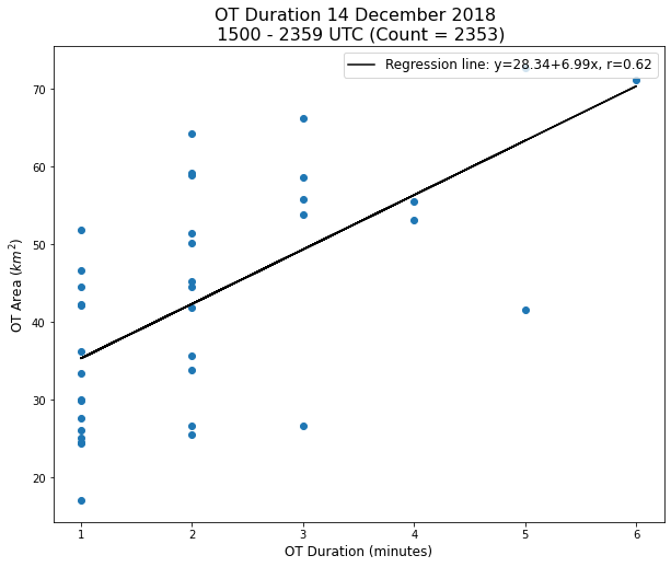
slope, intercept, r, p, stderr = scipy.stats.linregress(df_max.duration, df_max.area_polygon)

line = f'Regression line: y={intercept:.2f}+{slope:.2f}x, r={r:.2f}'

plt.figure(figsize=(10,8))
ax = plt.subplot(111)
ax.scatter(duration, max_otarea)
ax.plot(np.array(duration), intercept + slope * np.array(duration), label=line, color='black')

plt.ylabel('OT Area ($km^{2}$)', fontsize=12)
plt.xlabel('OT Duration (minutes)', fontsize=12)

plt.legend(loc='upper right', fontsize=12)

plt.title('OT Duration 14 December 2018 \n 0000 - 0635 UTC (Count = 710)', fontsize=16)

Text(0.5, 1.0, 'OT Duration 14 December 2018 \n 0000 - 0635 UTC (Count = 710)')

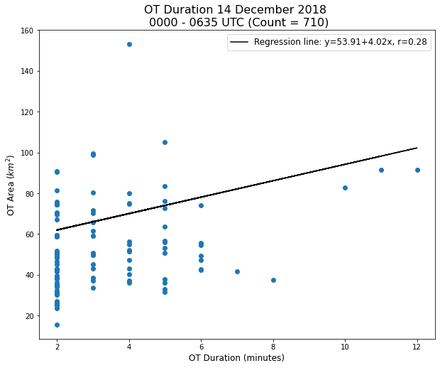
fig = plt.figure(figsize=(12,8))
plt.hist(df_max.area_polygon, bins=ota_bins)

plt.title('OTA Distribution \n 14 December 2018 0000-0635 UTC', fontsize=24)

plt.xlabel('OTA ($km^2$)', fontsize=16)
plt.ylabel('Frequency', fontsize=16)

Text(0, 0.5, 'Frequency')

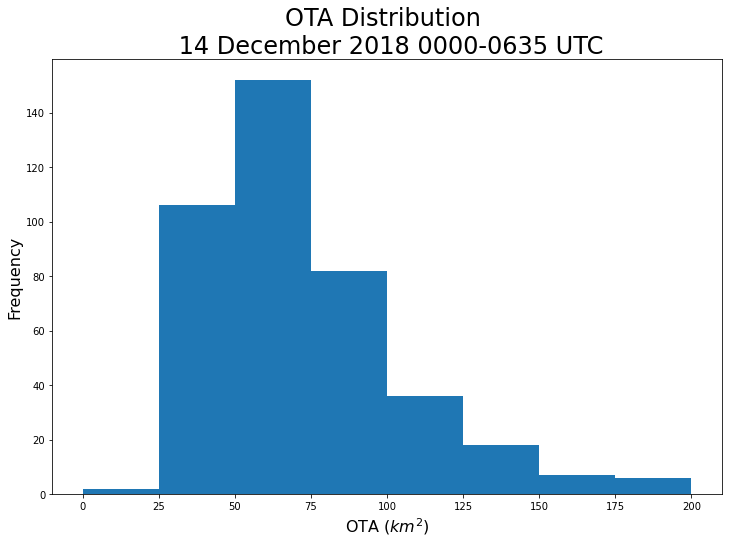
fig = plt.figure(figsize=(12,8))
plt.hist(df_max.ot_depth, bins=otd_bins)

plt.title('OT Depth Distribution \n 14 December 2018 0000-0635 UTC', fontsize=24)

plt.xlabel('OT Depth (km)', fontsize=16)
plt.ylabel('Frequency', fontsize=16)

Text(0, 0.5, 'Frequency')

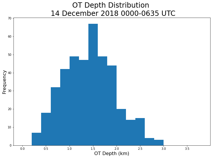
fig = plt.figure(figsize=(12,8))
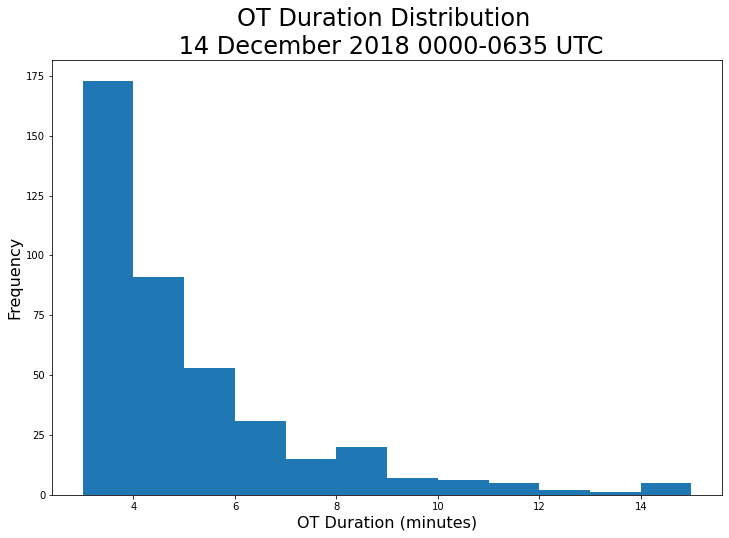
plt.hist(df_max.duration, bins=dur_bins)

plt.title('OT Duration Distribution \n 14 December 2018 0000-0635 UTC', fontsize=24)

plt.xlabel('OT Duration (minutes)', fontsize=16)
plt.ylabel('Frequency', fontsize=16)

Text(0, 0.5, 'Frequency')

llcrnr=[-33.206342, -65.906586]
urcrnr=[-30.255825, -62.630553]

# Set extent of maps created in the following cells:
#axis_extent=[llcrnr[1],urcrnr[1],llcrnr[0],urcrnr[0]]
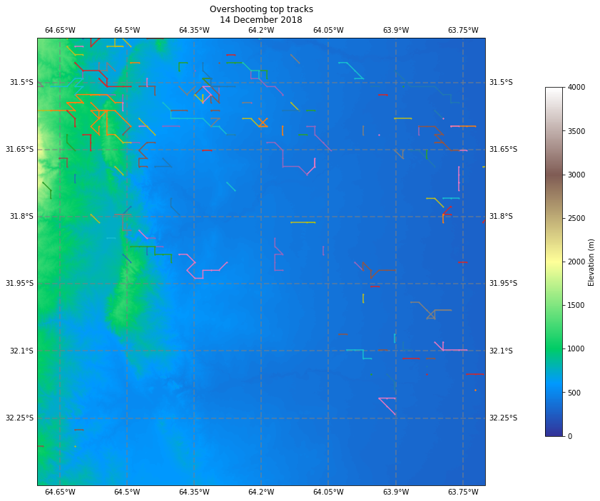
axis_extent=[-64.7, -63.7, -32.4, -31.4]  

# Plot map with all individual tracks:
import cartopy.crs as ccrs
fig_map,ax_map=plt.subplots(figsize=(15,15),subplot_kw={'projection': ccrs.PlateCarree()})

ax_map.coastlines()

ax_map.set_extent(axis_extent)

for ds in ds_list:
#    cm = ax.contourf(ds.x.values[::5], ds.y.values[::5], ds.values[::5,::5], levs, cmap='terrain', transform=ccrs.PlateCarree())
    cm = ax_map.imshow(ds.values, extent =[ds.x.min(),ds.x.max(),ds.y.min(),ds.y.max()], transform=ccrs.PlateCarree(), vmin=0, vmax=4000, cmap='terrain')

gl = ax_map.gridlines(crs=ccrs.PlateCarree(), draw_labels=True,
                  linewidth=2, color='gray', alpha=0.5, linestyle='--')

for name, group in cells_grouped:
#    print(group.x,group.y)
    plt.plot(group.lon,group.lat,"-o",markersize=1)

plt.colorbar(cm,label='Elevation (m)',shrink=0.6, pad=0.1)

ax_map.set_title('Overshooting top tracks\n14 December 2018')

Text(0.5, 1.0, 'Overshooting top tracks\n14 December 2018')

llcrnr=[-33.206342, -65.906586]
urcrnr=[-30.255825, -62.630553]

# Set extent of maps created in the following cells:
axis_extent=[llcrnr[1],urcrnr[1],llcrnr[0],urcrnr[0]]    

# Plot map with all individual tracks:
import cartopy.crs as ccrs
fig_map,ax_map=plt.subplots(figsize=(15,15),subplot_kw={'projection': ccrs.PlateCarree()})

ax_map.coastlines()

ax_map.set_extent(axis_extent)

for ds in ds_list:
#    cm = ax.contourf(ds.x.values[::5], ds.y.values[::5], ds.values[::5,::5], levs, cmap='terrain', transform=ccrs.PlateCarree())
    cm = ax_map.imshow(ds.values, extent =[ds.x.min(),ds.x.max(),ds.y.min(),ds.y.max()], transform=ccrs.PlateCarree(), vmin=0, vmax=4000, cmap='terrain')

gl = ax_map.gridlines(crs=ccrs.PlateCarree(), draw_labels=True,
                  linewidth=2, color='gray', alpha=0.5, linestyle='--')

for name, group in cells_grouped:
#    print(group.x,group.y)
    cm2 = plt.scatter(group.lon,group.lat,c=group.area_polygon,vmin=0.,vmax=200.,s=group.area_polygon,
                     facecolors='none',cmap='magma',linewidth=0.5)

plt.colorbar(cm,label='Elevation (m)',shrink=0.4, pad=0.0)
plt.colorbar(cm2,label='OT Area (km$^2$)',shrink=0.4, pad=0.1)



ax_map.set_title('Overshooting top tracks\n14 December 2018')

Text(0.5, 1.0, 'Overshooting top tracks\n14 December 2018')

---

All OTs

df = pd.concat([pd.read_csv(f) for f in sorted(glob.glob('ot_output/*/*'))], ignore_index = True).drop(columns='Unnamed: 0')

df['geometry'] = df['geometry'].apply(wkt.loads)
geo_df = gpd.GeoDataFrame(df, geometry='geometry')

df = geo_df
df['ot_depth'] = df.cloudtop_height - df.tropopause_height
df['btd'] = df.mintb - df.tropopause_temperature

df = df[df.ot_depth > 0]

df['diff'] = pd.to_datetime(df['time']) - pd.datetime(2018,11,1)
df['frame'] = df['diff'].dt.days*86400+df['diff'].dt.seconds
df['frame'] = df['frame'] - df['frame'].min()

df = df[df.prob > .8]

df_track = deepcopy(df)
#df_track.rename(columns={'lon':'x', 'lat':'y'}, inplace=True)
#df_track['z'] = 0
df_track['states'] = 0
df_track['label'] = 0

radius=6371228.

globe = ccrs.Globe(ellipse=None, semimajor_axis=radius, 
                   semiminor_axis=radius)

projection=ccrs.LambertAzimuthalEqualArea(central_latitude=-32.,
                                          central_longitude=-62.,globe=globe)

prj=pyproj.Proj(projection.proj4_init)

df_track['x'], df_track['y'] = prj(df_track['lon'].values, df_track['lat'].values)


df_track.to_csv('test.csv')

v_max=60.
stubs=2
order=1
extrapolate=1
memory=1
adaptive_stop=0.01
adaptive_step=0.99
subnetwork_size=100
method_linking= 'predict'
cell_number_start=1
dt = 60.
dxy = 2000.

search_range=dt*v_max

features_linking=deepcopy(df_track)

pred = tp.predict.NearestVelocityPredict(span=1)
trajectories_unfiltered = pred.link_df(features_linking, search_range=search_range, memory=memory,
                                 pos_columns=['x','y'],
                                 t_column='frame',
                                 neighbor_strategy='KDTree', link_strategy='auto',
                                 adaptive_step=adaptive_step,adaptive_stop=adaptive_stop
#                                 copy_features=False, diagnostics=False,
#                                 hash_size=None, box_size=None, verify_integrity=True,
#                                 retain_index=False
                                 )

trajectories_unfiltered['cell']=None
for i_particle,particle in enumerate(pd.Series.unique(trajectories_unfiltered['particle'])):
    cell=int(i_particle+cell_number_start)
    trajectories_unfiltered.loc[trajectories_unfiltered['particle']==particle,'cell']=cell
trajectories_unfiltered.drop(columns=['particle'],inplace=True)

trajectories_bycell=trajectories_unfiltered.groupby('cell')

num_stubs = 0

for cell,trajectories_cell in trajectories_bycell:
#    logging.debug("cell: "+str(cell))
#    logging.debug("feature: "+str(trajectories_cell['feature'].values))
#    logging.debug("trajectories_cell.shape[0]: "+ str(trajectories_cell.shape[0]))


    if trajectories_cell.shape[0] < stubs:
#        print("cell" + str(cell)+ "  is a stub ("+str(trajectories_cell.shape[0])+ "), setting cell number to Nan..")
        trajectories_unfiltered.loc[trajectories_unfiltered['cell']==cell,'cell']=np.nan
        num_stubs = num_stubs + 1

print('found this many stubs: {}'.format(num_stubs))

trajectories_filtered=trajectories_unfiltered.dropna(subset=['area_polygon', 'cell'])

Frame 2902710: 1 trajectories present.
found this many stubs: 974

df = trajectories_filtered

df['time'] = pd.to_datetime(trajectories_filtered.time)
df['day'] = df.time.dt.day
df['month'] = df.time.dt.month

/data/keeling/a/mgrover4/a/miniconda3/envs/xesmf_env/lib/python3.7/site-packages/ipykernel_launcher.py:3: SettingWithCopyWarning: 
A value is trying to be set on a copy of a slice from a DataFrame.
Try using .loc[row_indexer,col_indexer] = value instead

See the caveats in the documentation: https://pandas.pydata.org/pandas-docs/stable/user_guide/indexing.html#returning-a-view-versus-a-copy
  This is separate from the ipykernel package so we can avoid doing imports until
/data/keeling/a/mgrover4/a/miniconda3/envs/xesmf_env/lib/python3.7/site-packages/ipykernel_launcher.py:4: SettingWithCopyWarning: 
A value is trying to be set on a copy of a slice from a DataFrame.
Try using .loc[row_indexer,col_indexer] = value instead

See the caveats in the documentation: https://pandas.pydata.org/pandas-docs/stable/user_guide/indexing.html#returning-a-view-versus-a-copy
  after removing the cwd from sys.path.
/data/keeling/a/mgrover4/a/miniconda3/envs/xesmf_env/lib/python3.7/site-packages/ipykernel_launcher.py:5: SettingWithCopyWarning: 
A value is trying to be set on a copy of a slice from a DataFrame.
Try using .loc[row_indexer,col_indexer] = value instead

See the caveats in the documentation: https://pandas.pydata.org/pandas-docs/stable/user_guide/indexing.html#returning-a-view-versus-a-copy
  """

cells_grouped = df.groupby('cell')
df_max = cells_grouped.max()
df_min = cells_grouped.min()

df_max['duration']= cells_grouped.count().area_polygon
df_min['duration'] = cells_grouped.count().area_polygon

df_max = df_max[df_max.duration > 2]
df_min = df_min[df_min.duration > 2]

df_max['day'] = df_min.day

nov_10 = df_max[(df_max.day == 10) | (df_max.day == 11)]
nov_12 = df_max[df_max.day == 12]
dec_14 = df_max[(df_max.day == 14) | (df_max.day == 13)]

nov_10 = df[df.day == 10]
nov_12 = df[df.day == 12]
dec_14 = df[df.day == 14]

llcrnr=[-33.206342, -65.906586]
urcrnr=[-30.255825, -62.630553]

# Set extent of maps created in the following cells:
axis_extent=[-65, -63, -33, -31]     

# Plot map with all individual tracks:
import cartopy.crs as ccrs
fig_map,ax_map=plt.subplots(figsize=(12,8),subplot_kw={'projection': ccrs.PlateCarree()})
levs = np.arange(0, 2000, 100)

ax_map.coastlines()

ax_map.set_extent(axis_extent)

for ds in ds_list:
    cm = ax_map.contourf(ds.x.values[::5], ds.y.values[::5], ds.values[::5, ::5], levs, cmap='terrain', transform=ccrs.PlateCarree())


gl = ax_map.gridlines(crs=ccrs.PlateCarree(), draw_labels=True,
                  linewidth=2, color='gray', alpha=0.5, linestyle='--')
gl.top_labels = False
gl.left_labels= True
gl.right_labels = False
gl.xlabel_style = {'size': 16, 'color': 'k'}
gl.ylabel_style = {'size': 16, 'color': 'k'}

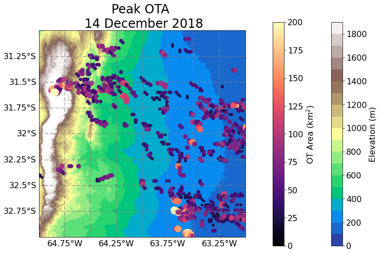
cm2 = plt.scatter(dec_14.lon.values,dec_14.lat.values,c=dec_14.area_polygon.values,vmin=0.,vmax=200.,s=dec_14.area_polygon,
                     facecolors='none',cmap='magma',linewidth=0.5)

cbar = plt.colorbar(cm, extend='both', label='Elevation (m)')
cbar.set_label(label='Elevation (m)', fontsize=16)
cbar.ax.tick_params(labelsize=16)

cbar2 = plt.colorbar(cm2,label='OT Area (km$^2$)', pad=0.1)
cbar2.set_label(label='OT Area (km$^2$)', fontsize=16)
cbar2.ax.tick_params(labelsize=16)



ax_map.set_title('Peak OTA \n 14 December 2018', fontsize=24)

/data/keeling/a/mgrover4/a/miniconda3/envs/xesmf_env/lib/python3.7/site-packages/ipykernel_launcher.py:31: MatplotlibDeprecationWarning: The 'extend' parameter to Colorbar has no effect because it is overridden by the mappable; it is deprecated since 3.3 and will be removed two minor releases later.

Text(0.5, 1.0, 'Peak OTA \n 14 December 2018')

llcrnr=[-33.206342, -65.906586]
urcrnr=[-30.255825, -62.630553]

# Set extent of maps created in the following cells:
axis_extent=[-65, -63, -33, -31]      

# Plot map with all individual tracks:
import cartopy.crs as ccrs
fig_map,ax_map=plt.subplots(figsize=(12,8),subplot_kw={'projection': ccrs.PlateCarree()})
levs = np.arange(0, 2000, 100)

ax_map.coastlines()

ax_map.set_extent(axis_extent)

for ds in ds_list:
    cm = ax_map.contourf(ds.x.values[::5], ds.y.values[::5], ds.values[::5, ::5], levs, cmap='terrain', transform=ccrs.PlateCarree())


gl = ax_map.gridlines(crs=ccrs.PlateCarree(), draw_labels=True,
                  linewidth=2, color='gray', alpha=0.5, linestyle='--')

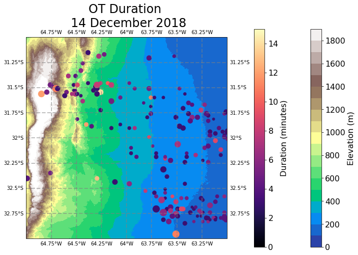
cm2 = plt.scatter(dec_14.lon.values,dec_14.lat.values,c=dec_14.duration.values,vmin=0.,vmax=15.,s=dec_14.area_polygon,
                     facecolors='none',cmap='magma',linewidth=0.5)

cbar = plt.colorbar(cm, extend='both', label='Elevation (m)')
cbar.set_label(label='Elevation (m)', fontsize=16)
cbar.ax.tick_params(labelsize=16)

cbar2 = plt.colorbar(cm2,label='OT Area (km$^2$)', pad=0.1)
cbar2.set_label(label='Duration (minutes)', fontsize=16)
cbar2.ax.tick_params(labelsize=16)



ax_map.set_title('OT Duration \n 14 December 2018', fontsize=24)

/data/keeling/a/mgrover4/a/miniconda3/envs/xesmf_env/lib/python3.7/site-packages/ipykernel_launcher.py:26: MatplotlibDeprecationWarning: The 'extend' parameter to Colorbar has no effect because it is overridden by the mappable; it is deprecated since 3.3 and will be removed two minor releases later.

Text(0.5, 1.0, 'OT Duration \n 14 December 2018')

llcrnr=[-33.206342, -65.906586]
urcrnr=[-30.255825, -62.630553]

# Plot map with all individual tracks:
import cartopy.crs as ccrs
fig_map,ax_map=plt.subplots(figsize=(12,8),subplot_kw={'projection': ccrs.PlateCarree()})
levs = np.arange(0, 2000, 100)

ax_map.coastlines()

ax_map.set_extent(axis_extent)

for ds in ds_list:
    cm = ax_map.contourf(ds.x.values[::5], ds.y.values[::5], ds.values[::5, ::5], levs, cmap='terrain', transform=ccrs.PlateCarree())


gl = ax_map.gridlines(crs=ccrs.PlateCarree(), draw_labels=True,
                  linewidth=2, color='gray', alpha=0.5, linestyle='--')
gl.top_labels = False
gl.left_labels= True
gl.right_labels = False
gl.xlabel_style = {'size': 16, 'color': 'k'}
gl.ylabel_style = {'size': 16, 'color': 'k'}

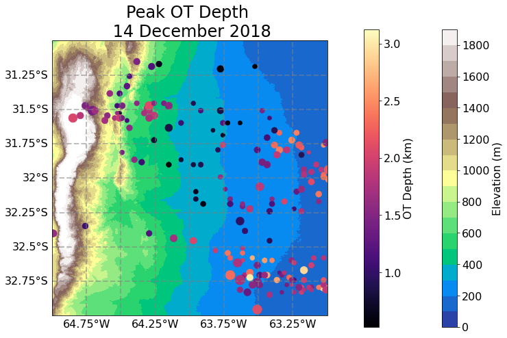
cm2 = plt.scatter(dec_14.lon.values,dec_14.lat.values,c=dec_14.ot_depth.values,s=dec_14.area_polygon,
                     facecolors='none',cmap='magma',linewidth=0.5)

cbar = plt.colorbar(cm, extend='both', label='Elevation (m)')
cbar.set_label(label='Elevation (m)', fontsize=16)
cbar.ax.tick_params(labelsize=16)

cbar2 = plt.colorbar(cm2,label='OT Area (km$^2$)', pad=0.1)
cbar2.set_label(label='OT Depth (km)', fontsize=16)
cbar2.ax.tick_params(labelsize=16)



ax_map.set_title('Peak OT Depth \n 14 December 2018', fontsize=24)

/data/keeling/a/mgrover4/a/miniconda3/envs/xesmf_env/lib/python3.7/site-packages/ipykernel_launcher.py:28: MatplotlibDeprecationWarning: The 'extend' parameter to Colorbar has no effect because it is overridden by the mappable; it is deprecated since 3.3 and will be removed two minor releases later.

Text(0.5, 1.0, 'Peak OT Depth \n 14 December 2018')

llcrnr=[-33.206342, -65.906586]
urcrnr=[-30.255825, -62.630553]

# Plot map with all individual tracks:
import cartopy.crs as ccrs
fig_map,ax_map=plt.subplots(figsize=(12,8),subplot_kw={'projection': ccrs.PlateCarree()})
levs = np.arange(0, 2000, 100)

ax_map.coastlines()

ax_map.set_extent(axis_extent)

for ds in ds_list:
    cm = ax_map.contourf(ds.x.values[::5], ds.y.values[::5], ds.values[::5, ::5], levs, cmap='terrain', transform=ccrs.PlateCarree())


gl = ax_map.gridlines(crs=ccrs.PlateCarree(), draw_labels=True,
                  linewidth=2, color='gray', alpha=0.5, linestyle='--')
gl.top_labels = False
gl.left_labels= True
gl.right_labels = False
gl.xlabel_style = {'size': 16, 'color': 'k'}
gl.ylabel_style = {'size': 16, 'color': 'k'} 

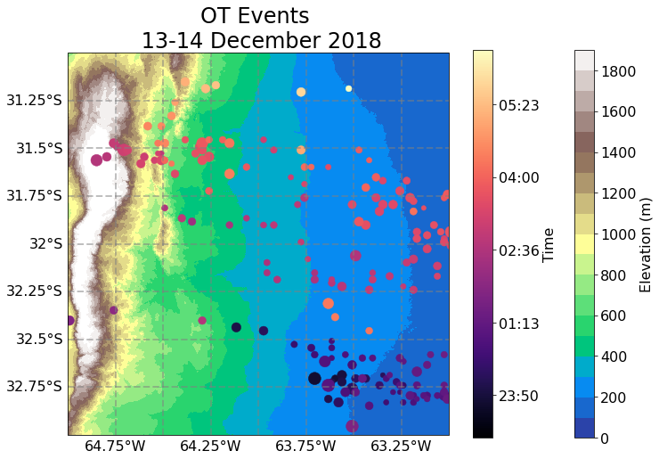
cm2 = plt.scatter(dec_14.lon.values,dec_14.lat.values,c=dec_14.time.values,s=dec_14.area_polygon,
                     facecolors='none',cmap='magma',linewidth=0.5)


# Change the numeric ticks into ones that match the x-axis


cbar = plt.colorbar(cm, extend='both', label='Elevation (m)')
cbar.set_label(label='Elevation (m)', fontsize=16)
cbar.ax.tick_params(labelsize=16)

cbar2 = plt.colorbar(cm2,label='OT Area (km$^2$)')
cbar2.set_label(label='Time', fontsize=16)
cbar2.ax.tick_params(labelsize=16)
cbar2.ax.set_yticklabels(pd.to_datetime(cbar2.get_ticks()).strftime(date_format='%H:%M'))



ax_map.set_title('OT Events \n 13-14 December 2018', fontsize=24)

/data/keeling/a/mgrover4/a/miniconda3/envs/xesmf_env/lib/python3.7/site-packages/ipykernel_launcher.py:32: MatplotlibDeprecationWarning: The 'extend' parameter to Colorbar has no effect because it is overridden by the mappable; it is deprecated since 3.3 and will be removed two minor releases later.
/data/keeling/a/mgrover4/a/miniconda3/envs/xesmf_env/lib/python3.7/site-packages/ipykernel_launcher.py:39: UserWarning: FixedFormatter should only be used together with FixedLocator

Text(0.5, 1.0, 'OT Events \n 13-14 December 2018')

llcrnr=[-33.206342, -65.906586]
urcrnr=[-30.255825, -62.630553]

# Set extent of maps created in the following cells:
axis_extent=[-65, -63, -33, -31]    

# Plot map with all individual tracks:
import cartopy.crs as ccrs
fig_map,ax_map=plt.subplots(figsize=(12,8),subplot_kw={'projection': ccrs.PlateCarree()})
levs = np.arange(0, 2000, 100)

ax_map.coastlines()

ax_map.set_extent(axis_extent)

for ds in ds_list:
    cm = ax_map.contourf(ds.x.values[::5], ds.y.values[::5], ds.values[::5, ::5], levs, cmap='terrain', transform=ccrs.PlateCarree())


gl = ax_map.gridlines(crs=ccrs.PlateCarree(), draw_labels=True,
                  linewidth=2, color='gray', alpha=0.5, linestyle='--')
gl.top_labels = False
gl.left_labels= True
gl.right_labels = False
gl.xlabel_style = {'size': 16, 'color': 'k'}
gl.ylabel_style = {'size': 16, 'color': 'k'}

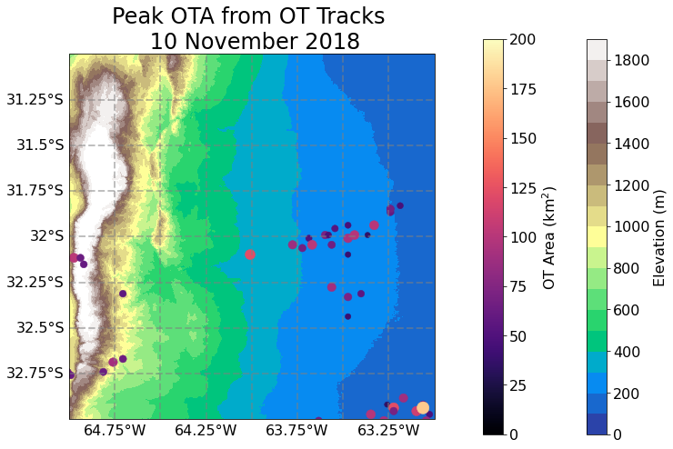
cm2 = plt.scatter(nov_10.lon.values,nov_10.lat.values,c=nov_10.area_polygon.values,vmin=0.,vmax=200.,s=nov_10.area_polygon,
                     facecolors='none',cmap='magma',linewidth=0.5)

cbar = plt.colorbar(cm, extend='both', label='Elevation (m)')
cbar.set_label(label='Elevation (m)', fontsize=16)
cbar.ax.tick_params(labelsize=16)

cbar2 = plt.colorbar(cm2,label='OT Area (km$^2$)', pad=0.1)
cbar2.set_label(label='OT Area (km$^2$)', fontsize=16)
cbar2.ax.tick_params(labelsize=16)



ax_map.set_title('Peak OTA from OT Tracks \n 10 November 2018', fontsize=24)

/data/keeling/a/mgrover4/a/miniconda3/envs/xesmf_env/lib/python3.7/site-packages/ipykernel_launcher.py:31: MatplotlibDeprecationWarning: The 'extend' parameter to Colorbar has no effect because it is overridden by the mappable; it is deprecated since 3.3 and will be removed two minor releases later.

Text(0.5, 1.0, 'Peak OTA from OT Tracks \n 10 November 2018')

llcrnr=[-33.206342, -65.906586]
urcrnr=[-30.255825, -62.630553] 

# Plot map with all individual tracks:
import cartopy.crs as ccrs
fig_map,ax_map=plt.subplots(figsize=(12,8),subplot_kw={'projection': ccrs.PlateCarree()})
levs = np.arange(0, 2000, 100)

ax_map.coastlines()

ax_map.set_extent(axis_extent)

for ds in ds_list:
    cm = ax_map.contourf(ds.x.values[::5], ds.y.values[::5], ds.values[::5, ::5], levs, cmap='terrain', transform=ccrs.PlateCarree())


gl = ax_map.gridlines(crs=ccrs.PlateCarree(), draw_labels=True,
                  linewidth=2, color='gray', alpha=0.5, linestyle='--')
gl.top_labels = False
gl.left_labels= True
gl.right_labels = False
gl.xlabel_style = {'size': 16, 'color': 'k'}
gl.ylabel_style = {'size': 16, 'color': 'k'}

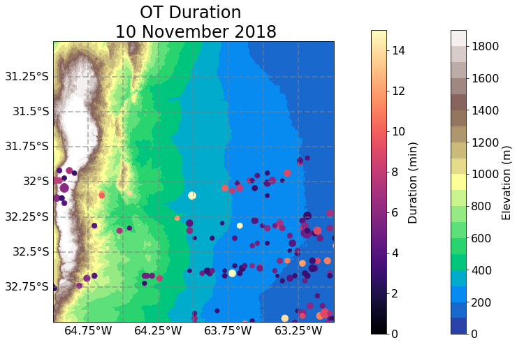
cm2 = plt.scatter(nov_10.lon.values,nov_10.lat.values,c=nov_10.duration.values,vmin=0.,vmax=15.,s=nov_10.area_polygon,
                     facecolors='none',cmap='magma',linewidth=0.5)

cbar = plt.colorbar(cm, extend='both', label='Elevation (m)')
cbar.set_label(label='Elevation (m)', fontsize=16)
cbar.ax.tick_params(labelsize=16)

cbar2 = plt.colorbar(cm2,label='OT Area (km$^2$)', pad=0.1)
cbar2.set_label(label='Duration (min)', fontsize=16)
cbar2.ax.tick_params(labelsize=16)



ax_map.set_title('OT Duration \n 10 November 2018', fontsize=24)

/data/keeling/a/mgrover4/a/miniconda3/envs/xesmf_env/lib/python3.7/site-packages/ipykernel_launcher.py:28: MatplotlibDeprecationWarning: The 'extend' parameter to Colorbar has no effect because it is overridden by the mappable; it is deprecated since 3.3 and will be removed two minor releases later.

Text(0.5, 1.0, 'OT Duration \n 10 November 2018')

llcrnr=[-33.206342, -65.906586]
urcrnr=[-30.255825, -62.630553] 

# Plot map with all individual tracks:
import cartopy.crs as ccrs
fig_map,ax_map=plt.subplots(figsize=(12,8),subplot_kw={'projection': ccrs.PlateCarree()})
levs = np.arange(0, 2000, 100)

ax_map.coastlines()

ax_map.set_extent(axis_extent)

for ds in ds_list:
    cm = ax_map.contourf(ds.x.values[::5], ds.y.values[::5], ds.values[::5, ::5], levs, cmap='terrain', transform=ccrs.PlateCarree())


gl = ax_map.gridlines(crs=ccrs.PlateCarree(), draw_labels=True,
                  linewidth=2, color='gray', alpha=0.5, linestyle='--')
gl.top_labels = False
gl.left_labels= True
gl.right_labels = False
gl.xlabel_style = {'size': 16, 'color': 'k'}
gl.ylabel_style = {'size': 16, 'color': 'k'}

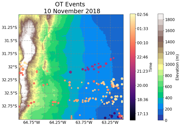
cm2 = plt.scatter(nov_10.lon.values,nov_10.lat.values,c=nov_10.time.values,s=nov_10.area_polygon,
                     facecolors='none',cmap='magma',linewidth=0.5)

cbar = plt.colorbar(cm, extend='both', label='Elevation (m)')
cbar.set_label(label='Elevation (m)', fontsize=16)
cbar.ax.tick_params(labelsize=16)

cbar2 = plt.colorbar(cm2,label='OT Area (km$^2$)')
cbar2.set_label(label='Time', fontsize=16)
cbar2.ax.tick_params(labelsize=16)
cbar2.ax.set_yticklabels(pd.to_datetime(cbar2.get_ticks()).strftime(date_format='%H:%M'))



ax_map.set_title('OT Events \n 10 November 2018', fontsize=24)

/data/keeling/a/mgrover4/a/miniconda3/envs/xesmf_env/lib/python3.7/site-packages/ipykernel_launcher.py:28: MatplotlibDeprecationWarning: The 'extend' parameter to Colorbar has no effect because it is overridden by the mappable; it is deprecated since 3.3 and will be removed two minor releases later.
/data/keeling/a/mgrover4/a/miniconda3/envs/xesmf_env/lib/python3.7/site-packages/ipykernel_launcher.py:35: UserWarning: FixedFormatter should only be used together with FixedLocator

Text(0.5, 1.0, 'OT Events \n 10 November 2018')

llcrnr=[-33.206342, -65.906586]
urcrnr=[-30.255825, -62.630553]
 

# Plot map with all individual tracks:
import cartopy.crs as ccrs
fig_map,ax_map=plt.subplots(figsize=(12,8),subplot_kw={'projection': ccrs.PlateCarree()})
levs = np.arange(0, 2000, 100)

ax_map.coastlines()

ax_map.set_extent(axis_extent)

for ds in ds_list:
    cm = ax_map.contourf(ds.x.values[::5], ds.y.values[::5], ds.values[::5, ::5], levs, cmap='terrain', transform=ccrs.PlateCarree())


gl = ax_map.gridlines(crs=ccrs.PlateCarree(), draw_labels=True,
                  linewidth=2, color='gray', alpha=0.5, linestyle='--')
gl.top_labels = False
gl.left_labels= True
gl.right_labels = False
gl.xlabel_style = {'size': 16, 'color': 'k'}
gl.ylabel_style = {'size': 16, 'color': 'k'}

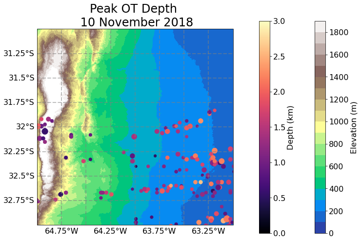
cm2 = plt.scatter(nov_10.lon.values,nov_10.lat.values,c=nov_10.ot_depth.values,vmin=0.,vmax=3.,s=nov_10.area_polygon,
                     facecolors='none',cmap='magma',linewidth=0.5)

cbar = plt.colorbar(cm, extend='both', label='Elevation (m)')
cbar.set_label(label='Elevation (m)', fontsize=16)
cbar.ax.tick_params(labelsize=16)

cbar2 = plt.colorbar(cm2,label='OT Area (km$^2$)', pad=0.1)
cbar2.set_label(label='Depth (km)', fontsize=16)
cbar2.ax.tick_params(labelsize=16)



ax_map.set_title('Peak OT Depth \n 10 November 2018', fontsize=24)

/data/keeling/a/mgrover4/a/miniconda3/envs/xesmf_env/lib/python3.7/site-packages/ipykernel_launcher.py:29: MatplotlibDeprecationWarning: The 'extend' parameter to Colorbar has no effect because it is overridden by the mappable; it is deprecated since 3.3 and will be removed two minor releases later.

Text(0.5, 1.0, 'Peak OT Depth \n 10 November 2018')

dec_14

	area_polygon	cloudtop_height	e_radial	e_radial_del2	e_tb	geometry	lat	lat_corr	lon	lon_corr	...	btd	diff	frame	states	label	x	y	cell	day	month
4353	27.820872	17.008001	2.512100	[ 0.15357971 0.16321182 0.05794525 -0.138183...	[197.50794983 198.54685974 199.89292908 201.27...	POLYGON ((-63.41965 -32.72321, -63.40088 -32.7...	-32.687500	-32.564499	-63.419647	-63.465649	...	-7.050003	43 days 00:00:25.000000512	2879071	0	0	-132858.256112	-77325.241389	958	14	12
4354	45.744502	17.170000	5.021842	[ 0.26845551 0.35186768 0.3476181 0.193073...	[196.36286926 195.73219299 195.63842773 195.87...	POLYGON ((-63.63393 -32.76786, -63.60579 -32.7...	-32.723213	-32.599213	-63.633930	-63.679932	...	-8.329987	43 days 00:00:25.000000512	2879071	0	0	-152848.759870	-81580.793324	959	14	12
4356	35.420817	17.276001	3.344912	[ 0.41732788 0.53477859 0.48075867 0.159931...	[196.95626831 197.06828308 198.01495361 199.43...	POLYGON ((-63.63393 -32.85714, -63.60109 -32.8...	-32.812500	-32.687500	-63.633930	-63.679932	...	-9.210007	43 days 00:00:25.000000512	2879071	0	0	-152696.307625	-91508.748519	960	14	12
4357	33.917275	16.268002	3.335197	[ 0.2013855 0.27927017 0.29254532 0.144180...	[203.81013489 203.84004211 204.27272034 205.01...	POLYGON ((-65.06250 -33.10714, -65.04374 -33.0...	-33.080357	-32.962357	-65.062500	-65.100502	...	-5.000000	43 days 00:00:25.000000512	2879071	0	0	-285295.264231	-124204.623051	957	14	12
4358	57.817719	17.937000	4.996009	[ 2.07168579e-01 2.75302887e-01 2.85362244e-...	[191.43812561 191.50009155 191.97639465 192.72...	POLYGON ((-62.77679 -33.19926, -62.76740 -33.1...	-33.187500	-33.055500	-62.776787	-62.828785	...	-12.600006	43 days 00:00:25.000000512	2879071	0	0	-72291.077516	-132308.177974	952	14	12
...	...	...	...	...	...	...	...	...	...	...	...	...	...	...	...	...	...	...	...	...	...
7837	45.825843	16.686001	5.000000	[ 0.16270447 0.23226547 0.25936508 0.153068...	[195.18452454 195.12481689 195.39051819 195.93...	POLYGON ((-67.61607 -27.00000, -67.58793 -26.9...	-31.205359	-26.955357	-63.526783	-67.616074	...	-2.039993	43 days 06:25:25.000000512	2902171	0	0	-145208.263845	87342.890014	1949	14	12
7840	24.486986	17.549002	3.000000	[94.7826767 94.7826767 47.39133835 0. ...	[189.56535339 0. 0. 0. ...	POLYGON ((-66.72322 -26.75000, -66.70914 -26.7...	-30.973215	-26.723215	-62.633926	-66.723221	...	-7.099991	43 days 06:27:25.000000512	2902291	0	0	-60442.164268	113999.920948	1951	14	12
7843	30.263209	17.159000	3.000000	[95.89810181 95.89810181 47.9490509 0. ...	[191.79620361 0. 0. 0. ...	POLYGON ((-66.72322 -26.74107, -66.70914 -26.7...	-30.955357	-26.705357	-62.633926	-66.723221	...	-4.589996	43 days 06:28:25.000000512	2902351	0	0	-60453.554044	115985.618850	1951	14	12
7856	59.017049	16.591002	4.000000	[ 0.10934448 0.14450455 0.13109207 0.027835...	[195.60501099 195.75 196.11367798 196.61...	POLYGON ((-67.66964 -26.87500, -67.64619 -26.8...	-31.080357	-26.830359	-63.580360	-67.669640	...	-1.300003	43 days 06:32:25.000000512	2902591	0	0	-150502.769321	101169.280988	1954	14	12
7858	61.092856	16.749001	4.000000	[ 0.13513947 0.17360687 0.14691925 0.013507...	[194.45181274 194.74206543 195.30259705 196.01...	POLYGON ((-67.63393 -26.88393, -67.61048 -26.8...	-31.080357	-26.830359	-63.544643	-67.633926	...	-2.339996	43 days 06:34:24.999999488	2902710	0	0	-147101.703963	101218.124030	1954	14	12

1608 rows × 49 columns

Linear Regression

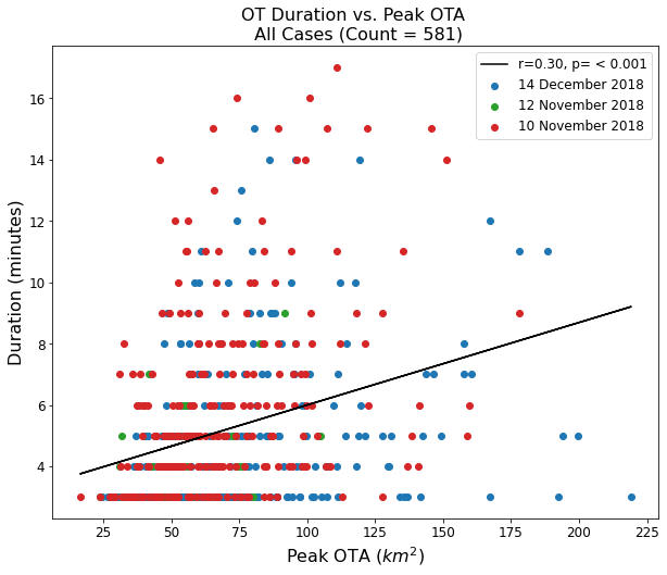
slope, intercept, r, p, stderr = scipy.stats.linregress(df_max.area_polygon, df_max.duration)

line = f'r={r:.2f}, p= < 0.001'

plt.figure(figsize=(10,8))
ax = plt.subplot(111)

#max_depth_nov_10 = max_depth[max_depth.day == 10]
ax.scatter(dec_14.area_polygon, dec_14.duration, color='tab:blue', label='14 December 2018')
ax.scatter(nov_12.area_polygon, nov_12.duration, color='tab:green', label='12 November 2018')
ax.scatter(nov_10.area_polygon, nov_10.duration, color='tab:red', label='10 November 2018')

#ax.scatter(np.median(dec_14.duration), np.median(dec_14.area_polygon), color='blue', s=100)
#ax.scatter(np.median(nov_10.duration), np.median(nov_10.area_polygon), color='red', s=100)
#ax.scatter(np.median(nov_12.duration), np.median(nov_12.area_polygon), color='green', s=100)

#ax.scatter(np.mean(dec_14.duration), np.mean(dec_14.area_polygon), color='blue', s=100)
#ax.scatter(np.mean(nov_10.duration), np.mean(nov_10.area_polygon), color='red', s=100)
#ax.scatter(np.mean(nov_12.duration), np.mean(nov_12.area_polygon), color='green', s=100)



ax.plot(np.array(df_max.area_polygon), intercept + slope * np.array(df_max.area_polygon), label=line, color='black')

plt.ylabel('Duration (minutes)', fontsize=16)
plt.xlabel('Peak OTA ($km^{2}$)', fontsize=16)

plt.legend(loc='upper right', fontsize=12)

plt.xticks(fontsize=12)
plt.yticks(fontsize=12)

plt.title(f'OT Duration vs. Peak OTA \n All Cases (Count = {len(df_max)})', fontsize=16)

plt.savefig('OT_duration_Peak_OTA.png', dpi=300)

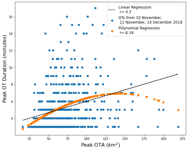
from sklearn.metrics import r2_score
x = df_max.area_polygon
y = df_max.duration

mymodel = numpy.poly1d(np.polyfit(x, y, 3))
linmodel = numpy.poly1d(np.polyfit(x, y, 1))

r_poly = np.sqrt(r2_score(y, mymodel(x)))
r_lin = np.sqrt(r2_score(y, linmodel(x)))

fig = plt.figure(figsize=(10, 8))
plt.scatter(x, y, label='OTs from 10 November, \n 12 November, 14 December 2018')
plt.scatter(x, mymodel(x), label=f'Polynomial Regression \n r= {round(r_poly, 2)}')
plt.plot(x, linmodel(x), linestyle='--', color='k', label=f'Linear Regression \n r= {round(r_lin, 2)}')
plt.legend(loc='upper right', fontsize=12)

plt.xlabel('Peak OTA ($km^2$)', fontsize=16)
plt.ylabel('Peak OT Duration ($minutes$)', fontsize=16)

Text(0, 0.5, 'Peak OT Duration ($minutes$)')

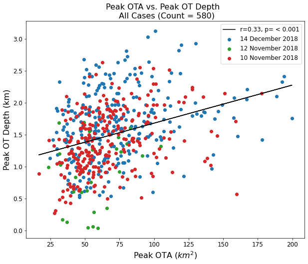
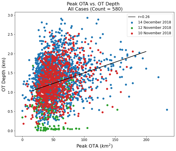
slope, intercept, r, p, stderr = scipy.stats.linregress(df_max.area_polygon, df_max.ot_depth)

line = f'r={r:.2f}, p= < 0.001'

plt.figure(figsize=(10,8))
ax = plt.subplot(111)

#max_depth_nov_10 = max_depth[max_depth.day == 10]
ax.scatter(dec_14.area_polygon, dec_14.ot_depth, color='tab:blue', label='14 December 2018')
ax.scatter(nov_12.area_polygon, nov_12.ot_depth, color='tab:green', label='12 November 2018')
ax.scatter(nov_10.area_polygon, nov_10.ot_depth, color='tab:red', label='10 November 2018')

#ax.scatter(np.median(dec_14.area_polygon), np.median(dec_14.ot_depth), color='blue', s=100)
#ax.scatter(np.median(nov_10.area_polygon), np.median(nov_10.ot_depth), color='red', s=100)
#ax.scatter(np.median(nov_12.area_polygon), np.median(nov_12.ot_depth), color='green', s=100)

ax.plot(np.array(df_max.area_polygon), intercept + slope * np.array(df_max.area_polygon), label=line, color='black')

plt.xlabel('Peak OTA ($km^{2}$)', fontsize=16)
plt.ylabel('Peak OT Depth (km)', fontsize=16)

plt.legend(loc='upper right', fontsize=12)

plt.xticks(fontsize=12)
plt.yticks(fontsize=12)

plt.title(f'Peak OTA vs. Peak OT Depth  \n All Cases (Count = {len(df_max)})', fontsize=16)
plt.savefig('OTA_OT_Depth.png', dpi=300)

slope, intercept, r, p, stderr = scipy.stats.linregress(df_max.area_polygon, df_max.ot_depth)

nov_10_min = df_min[df_min.day == 10]
nov_12_min = df_min[df_min.day == 12]
dec_14_min = df_min[df_min.day == 14]

slope, intercept, r, p, stderr = scipy.stats.linregress(df_min.btd, df_max.ot_depth)

line = f'r={r:.2f}'

plt.figure(figsize=(10,8))
ax = plt.subplot(111)
#max_depth_nov_10 = max_depth[max_depth.day == 10]
ax.scatter(dec_14_min.btd, dec_14.ot_depth, color='tab:blue', label='14 December 2018')
ax.scatter(nov_12_min.btd, nov_12.ot_depth, color='tab:green', label='12 November 2018')
ax.scatter(nov_10_min.btd, nov_10.ot_depth, color='tab:red', label='10 November 2018')

ax.scatter(np.median(dec_14_min.btd), np.median(dec_14.ot_depth), color='blue', s=100)
ax.scatter(np.median(nov_10_min.btd), np.median(nov_10.ot_depth), color='red', s=100)
ax.scatter(np.median(nov_12_min.btd), np.median(nov_12.ot_depth), color='green', s=100)

ax.plot(np.array(df_min.btd), intercept + slope * np.array(df_min.btd), label=line, color='black')

plt.xlabel('BTD (IR Temp - Trop Temp) (K)', fontsize=12)
plt.ylabel('OT Depth (km)', fontsize=12)

plt.legend(loc='upper right', fontsize=12)

plt.title('OT BTD vs. OT Depth  \n 10 November, 12 November, 14 December 2018 UTC (Count = 579)', fontsize=16)

---------------------------------------------------------------------------
ValueError                                Traceback (most recent call last)
<ipython-input-24-2390c796d286> in <module>
      6 ax = plt.subplot(111)
      7 #max_depth_nov_10 = max_depth[max_depth.day == 10]
----> 8 ax.scatter(dec_14_min.btd, dec_14.ot_depth, color='tab:blue', label='14 December 2018')
      9 ax.scatter(nov_12_min.btd, nov_12.ot_depth, color='tab:green', label='12 November 2018')
     10 ax.scatter(nov_10_min.btd, nov_10.ot_depth, color='tab:red', label='10 November 2018')

~/a/miniconda3/envs/xesmf_env/lib/python3.7/site-packages/matplotlib/__init__.py in inner(ax, data, *args, **kwargs)
   1436     def inner(ax, *args, data=None, **kwargs):
   1437         if data is None:
-> 1438             return func(ax, *map(sanitize_sequence, args), **kwargs)
   1439 
   1440         bound = new_sig.bind(ax, *args, **kwargs)

~/a/miniconda3/envs/xesmf_env/lib/python3.7/site-packages/matplotlib/cbook/deprecation.py in wrapper(*inner_args, **inner_kwargs)
    409                          else deprecation_addendum,
    410                 **kwargs)
--> 411         return func(*inner_args, **inner_kwargs)
    412 
    413     return wrapper

~/a/miniconda3/envs/xesmf_env/lib/python3.7/site-packages/matplotlib/axes/_axes.py in scatter(self, x, y, s, c, marker, cmap, norm, vmin, vmax, alpha, linewidths, verts, edgecolors, plotnonfinite, **kwargs)
   4439         y = np.ma.ravel(y)
   4440         if x.size != y.size:
-> 4441             raise ValueError("x and y must be the same size")
   4442 
   4443         if s is None:

ValueError: x and y must be the same size

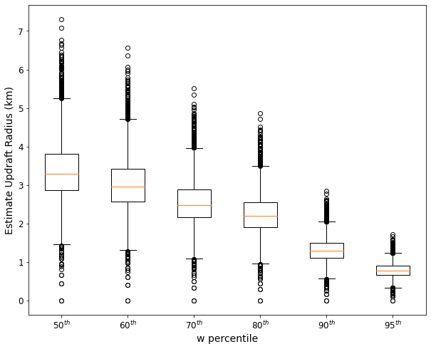
def calc_r(area, scale=0.412):
    
    return np.sqrt(area*scale/np.pi) 

df['mid_ur_50'] = calc_r(df['area_polygon'], 0.72)
df['mid_ur_60'] = calc_r(df['area_polygon'], 0.58)
df['mid_ur_70'] = calc_r(df['area_polygon'], 0.41)
df['mid_ur_80'] = calc_r(df['area_polygon'], 0.32)
df['mid_ur_90'] = calc_r(df['area_polygon'], 0.11)
df['mid_ur_95'] = calc_r(df['area_polygon'], 0.04)
df['mid_ud'] = calc_r(df['area_polygon']) * 2

/data/keeling/a/mgrover4/a/miniconda3/envs/xesmf_env/lib/python3.7/site-packages/ipykernel_launcher.py:1: SettingWithCopyWarning: 
A value is trying to be set on a copy of a slice from a DataFrame.
Try using .loc[row_indexer,col_indexer] = value instead

See the caveats in the documentation: https://pandas.pydata.org/pandas-docs/stable/user_guide/indexing.html#returning-a-view-versus-a-copy
  """Entry point for launching an IPython kernel.
/data/keeling/a/mgrover4/a/miniconda3/envs/xesmf_env/lib/python3.7/site-packages/ipykernel_launcher.py:2: SettingWithCopyWarning: 
A value is trying to be set on a copy of a slice from a DataFrame.
Try using .loc[row_indexer,col_indexer] = value instead

See the caveats in the documentation: https://pandas.pydata.org/pandas-docs/stable/user_guide/indexing.html#returning-a-view-versus-a-copy
  
/data/keeling/a/mgrover4/a/miniconda3/envs/xesmf_env/lib/python3.7/site-packages/ipykernel_launcher.py:3: SettingWithCopyWarning: 
A value is trying to be set on a copy of a slice from a DataFrame.
Try using .loc[row_indexer,col_indexer] = value instead

See the caveats in the documentation: https://pandas.pydata.org/pandas-docs/stable/user_guide/indexing.html#returning-a-view-versus-a-copy
  This is separate from the ipykernel package so we can avoid doing imports until
/data/keeling/a/mgrover4/a/miniconda3/envs/xesmf_env/lib/python3.7/site-packages/ipykernel_launcher.py:4: SettingWithCopyWarning: 
A value is trying to be set on a copy of a slice from a DataFrame.
Try using .loc[row_indexer,col_indexer] = value instead

See the caveats in the documentation: https://pandas.pydata.org/pandas-docs/stable/user_guide/indexing.html#returning-a-view-versus-a-copy
  after removing the cwd from sys.path.
/data/keeling/a/mgrover4/a/miniconda3/envs/xesmf_env/lib/python3.7/site-packages/ipykernel_launcher.py:5: SettingWithCopyWarning: 
A value is trying to be set on a copy of a slice from a DataFrame.
Try using .loc[row_indexer,col_indexer] = value instead

See the caveats in the documentation: https://pandas.pydata.org/pandas-docs/stable/user_guide/indexing.html#returning-a-view-versus-a-copy
  """
/data/keeling/a/mgrover4/a/miniconda3/envs/xesmf_env/lib/python3.7/site-packages/ipykernel_launcher.py:6: SettingWithCopyWarning: 
A value is trying to be set on a copy of a slice from a DataFrame.
Try using .loc[row_indexer,col_indexer] = value instead

See the caveats in the documentation: https://pandas.pydata.org/pandas-docs/stable/user_guide/indexing.html#returning-a-view-versus-a-copy
  
/data/keeling/a/mgrover4/a/miniconda3/envs/xesmf_env/lib/python3.7/site-packages/ipykernel_launcher.py:7: SettingWithCopyWarning: 
A value is trying to be set on a copy of a slice from a DataFrame.
Try using .loc[row_indexer,col_indexer] = value instead

See the caveats in the documentation: https://pandas.pydata.org/pandas-docs/stable/user_guide/indexing.html#returning-a-view-versus-a-copy
  import sys

figure = plt.figure(figsize=(10,8))
plt.boxplot([df.mid_ur_50, df.mid_ur_60, df.mid_ur_70, df.mid_ur_80, df.mid_ur_90, df.mid_ur_95])
plt.xticks([1, 2, 3, 4, 5, 6], ['$50^{th}$', '$60^{th}$', '$70^{th}$', '$80^{th}$', '$90^{th}$', '$95^{th}$'], fontsize=12)

plt.ylabel('Estimate Updraft Radius (km)', fontsize=14)
plt.xlabel('w percentile', fontsize=14)

plt.yticks(fontsize=12)

(array([-1.,  0.,  1.,  2.,  3.,  4.,  5.,  6.,  7.,  8.]),
 [Text(0, 0, ''),
  Text(0, 0, ''),
  Text(0, 0, ''),
  Text(0, 0, ''),
  Text(0, 0, ''),
  Text(0, 0, ''),
  Text(0, 0, ''),
  Text(0, 0, ''),
  Text(0, 0, ''),
  Text(0, 0, '')])

p

0.0

np.median(df.mid_ur_60)

2.9573037952551773

np.median(df.mid_ur_70)

2.486416460368345

np.median(df.mid_ur_80)

2.196630113408756

np.median(df.mid_ur_90) * 2

2.5757771256087896

np.median(df.mid_ur_95) * 2

1.5532520489499064

plt.hist()

---------------------------------------------------------------------------
TypeError                                 Traceback (most recent call last)
<ipython-input-34-85881ad87f6d> in <module>
----> 1 plt.hist()

TypeError: hist() missing 1 required positional argument: 'x'

df['est_wmax'] = df['ot_depth'] * 34.234

/data/keeling/a/mgrover4/a/miniconda3/envs/xesmf_env/lib/python3.7/site-packages/ipykernel_launcher.py:1: SettingWithCopyWarning: 
A value is trying to be set on a copy of a slice from a DataFrame.
Try using .loc[row_indexer,col_indexer] = value instead

See the caveats in the documentation: https://pandas.pydata.org/pandas-docs/stable/user_guide/indexing.html#returning-a-view-versus-a-copy
  """Entry point for launching an IPython kernel.

nov_10 = df[df.day == 10]
nov_12 = df[df.day == 12]
dec_14 = df[df.day == 14]

df_mean = df.groupby('cell').mean()
df_max = df.groupby('cell').max()

df_max['duration']= cells_grouped.count().area_polygon
df_mean['duration'] = cells_grouped.count().area_polygon

df_max = df_max[df_max.duration > 2]
df_mean = df_mean[df_mean.duration > 2]

nov_10_mean = df_mean[df_mean.day == 10]
nov_12_mean = df_mean[df_mean.day == 12]
dec_14_mean = df_mean[df_mean.day == 14]

nov_10_max = df_max[df_max.day == 10]
nov_12_max = df_max[df_max.day == 12]
dec_14_max = df_max[df_max.day == 14]

slope, intercept, r, p, stderr = scipy.stats.linregress(df.area_polygon, df.ot_depth)

line = f'r={r:.2f}'

plt.figure(figsize=(10,8))
ax = plt.subplot(111)

#max_depth_nov_10 = max_depth[max_depth.day == 10]
ax.scatter(dec_14.area_polygon, dec_14.ot_depth, color='tab:blue', label='14 December 2018')
ax.scatter(nov_12.area_polygon, nov_12.ot_depth, color='tab:green', label='12 November 2018')
ax.scatter(nov_10.area_polygon, nov_10.ot_depth, color='tab:red', label='10 November 2018')

#ax.scatter(np.median(dec_14.area_polygon), np.median(dec_14.ot_depth), color='blue', s=100)
#ax.scatter(np.median(nov_10.area_polygon), np.median(nov_10.ot_depth), color='red', s=100)
#ax.scatter(np.median(nov_12.area_polygon), np.median(nov_12.ot_depth), color='green', s=100)

ax.plot(np.array(df_max.area_polygon), intercept + slope * np.array(df_max.area_polygon), label=line, color='black')

plt.xlabel('Peak OTA ($km^{2}$)', fontsize=16)
plt.ylabel('OT Depth (km)', fontsize=16)

plt.legend(loc='upper right', fontsize=12)

plt.xticks(fontsize=12)
plt.yticks(fontsize=12)

plt.title(f'Peak OTA vs. OT Depth  \n All Cases (Count = {len(df_max)})', fontsize=16)
plt.savefig('OTA_OT_Depth.png', dpi=300)

nov_10_max.duration.mean()

5.948717948717949

u_core_bins = np.arange(0, 6.25, .25)
ua_bins = np.arange(0, 100, 10)
otw_bins = np.arange(0, 10.5, .5)

fig = plt.figure(figsize=(20,8))


ax = plt.subplot(121)
ax.hist(dec_14_max.area_polygon, ota_bins, label='14 Dec', color='white',
        edgecolor='tab:blue', linewidth=3)
ax.hist(nov_10_max.area_polygon, ota_bins, label='10 Nov', color='white',
        edgecolor='tab:red', linewidth=3)
ax.hist(nov_12_max.area_polygon, ota_bins, label='12 Nov', color='white',
        edgecolor='tab:green', linewidth=3)


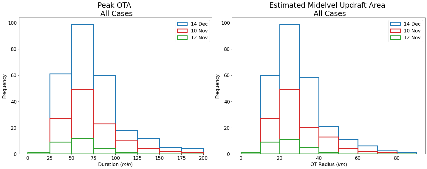
plt.title('Peak OTA \n All Cases', fontsize=24)

plt.xlabel('Duration ($min$)', fontsize=16)
plt.ylabel('Frequency', fontsize=16)

plt.xticks(fontsize=16)
plt.yticks(fontsize=16)
plt.legend(loc='upper right', fontsize=16)

ax2 = plt.subplot(122)
#plt.hist(df_max.area_polygon * 0.4032)



ax2.hist((dec_14_max.area_polygon* 0.4032), ua_bins, label='14 Dec', color='white',
         edgecolor='tab:blue', linewidth=3)
ax2.hist((nov_10_max.area_polygon * 0.4032), ua_bins, label='10 Nov', color='white',
         edgecolor='tab:red', linewidth=3)
ax2.hist((nov_12_max.area_polygon * 0.4032), ua_bins, label='12 Nov', color='white',
         edgecolor='tab:green', linewidth=3)


plt.title('Estimated Midelvel Updraft Area \n All Cases', fontsize=24)

plt.xlabel('OT Radius ($km$)', fontsize=16)
plt.ylabel('Frequency', fontsize=16)

plt.xticks(fontsize=16)
plt.yticks(fontsize=16)

plt.legend(loc='upper right', fontsize=16)

plt.tight_layout()
plt.savefig('OTA_Radius.png', dpi=300)

u_core_bins = np.arange(0, 6.25, .25)
ua_bins = np.arange(0, 100, 10)
otw_bins = np.arange(0, 10.5, .5)

fig = plt.figure(figsize=(20,8))


ax = plt.subplot(121)
ax.hist(dec_14_max.area_polygon, ota_bins, label='14 Dec', color='white',
        edgecolor='tab:blue', linewidth=3)
ax.hist(nov_10_max.area_polygon, ota_bins, label='10 Nov', color='white',
        edgecolor='tab:red', linewidth=3)
ax.hist(nov_12_max.area_polygon, ota_bins, label='12 Nov', color='white',
        edgecolor='tab:green', linewidth=3)


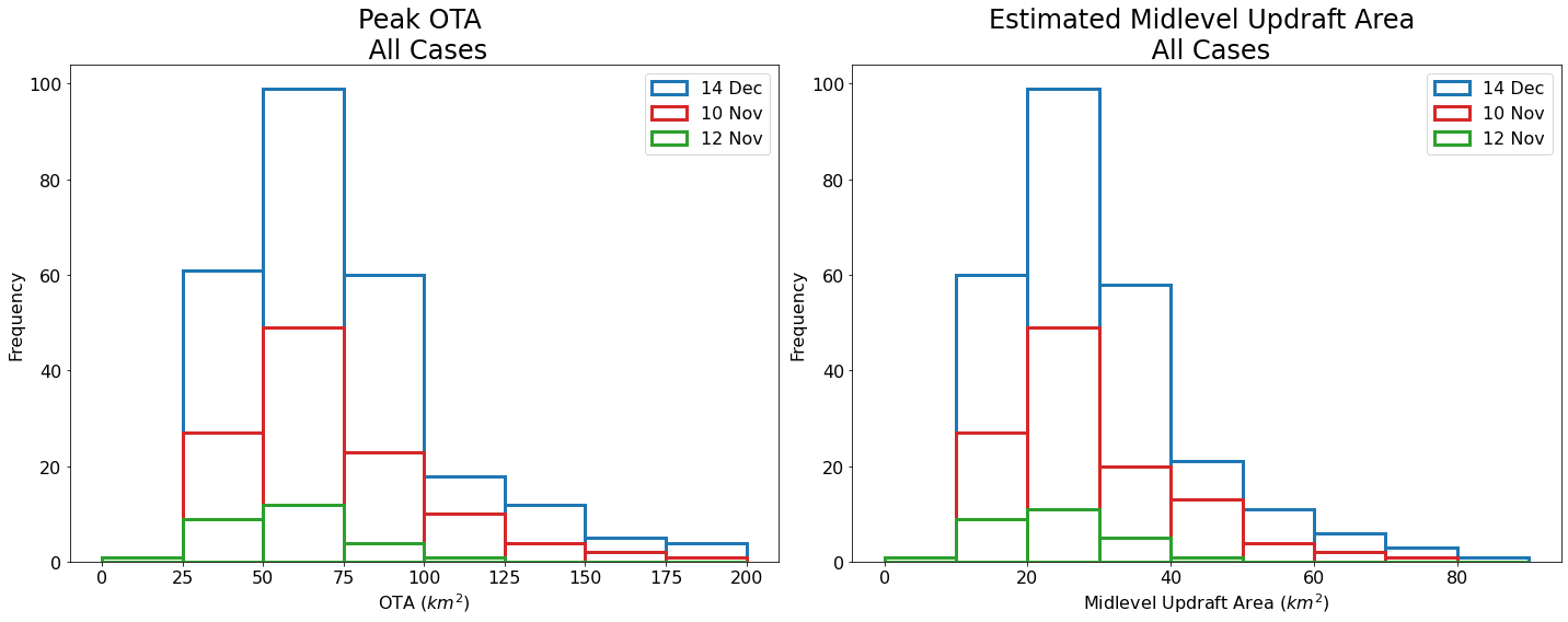
plt.title('Peak OTA \n All Cases', fontsize=24)

plt.xlabel('OTA ($km^2$)', fontsize=16)
plt.ylabel('Frequency', fontsize=16)

plt.xticks(fontsize=16)
plt.yticks(fontsize=16)
plt.legend(loc='upper right', fontsize=16)

ax2 = plt.subplot(122)
#plt.hist(df_max.area_polygon * 0.4032)



ax2.hist((dec_14_max.area_polygon* 0.4032), ua_bins, label='14 Dec', color='white',
         edgecolor='tab:blue', linewidth=3)
ax2.hist((nov_10_max.area_polygon * 0.4032), ua_bins, label='10 Nov', color='white',
         edgecolor='tab:red', linewidth=3)
ax2.hist((nov_12_max.area_polygon * 0.4032), ua_bins, label='12 Nov', color='white',
         edgecolor='tab:green', linewidth=3)


plt.title('Estimated Midlevel Updraft Area \n All Cases', fontsize=24)

plt.xlabel('Midlevel Updraft Area ($km^2$)', fontsize=16)
plt.ylabel('Frequency', fontsize=16)

plt.xticks(fontsize=16)
plt.yticks(fontsize=16)

plt.legend(loc='upper right', fontsize=16)

plt.tight_layout()
plt.savefig('OTA_Radius.png', dpi=300)

ota_ua_scale = 0.4032

u_core_bins = np.arange(0, 6.25, .25)
ua_bins = np.arange(0, 100, 10)
otw_bins = np.arange(0, 10.5, .5)

fig = plt.figure(figsize=(20,8))


ax = plt.subplot(121)
ax.hist(dec_14_max.duration, dur_bins, label='14 Dec', color='white',
        edgecolor='tab:blue', linewidth=3)
ax.hist(nov_10_max.duration, dur_bins, label='10 Nov', color='white',
        edgecolor='tab:red', linewidth=3)
ax.hist(nov_12_max.duration, dur_bins, label='12 Nov', color='white',
        edgecolor='tab:green', linewidth=3)


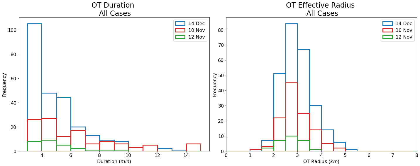
plt.title('OT Duration \n All Cases', fontsize=24)

plt.xlabel('Duration ($min$)', fontsize=16)
plt.ylabel('Frequency', fontsize=16)

plt.xticks(fontsize=16)
plt.yticks(fontsize=16)
plt.legend(loc='upper right', fontsize=16)

ax2 = plt.subplot(122)
#plt.hist(df_max.area_polygon * 0.4032)



ax2.hist(calc_r(dec_14_max.area_polygon,ota_ua_scale), otw_bins, label='14 Dec', color='white',
         edgecolor='tab:blue', linewidth=3)
ax2.hist(calc_r(nov_10_max.area_polygon,ota_ua_scale), otw_bins, label='10 Nov', color='white',
         edgecolor='tab:red', linewidth=3)
ax2.hist(calc_r(nov_12_max.area_polygon,ota_ua_scale), otw_bins, label='12 Nov', color='white',
         edgecolor='tab:green', linewidth=3)

plt.xlim(0, 8)


plt.title('OT Effective Radius \n All Cases', fontsize=24)

plt.xlabel('OT Radius ($km$)', fontsize=16)
plt.ylabel('Frequency', fontsize=16)

plt.xticks(fontsize=16)
plt.yticks(fontsize=16)

plt.legend(loc='upper right', fontsize=16)

plt.tight_layout()
plt.savefig('OT_Duration_Radius.png', dpi=300)

np.median(df.area_polygon * 0.4032)

19.10004031090206

np.median(df.area_polygon * 0.44)

20.84329795832566

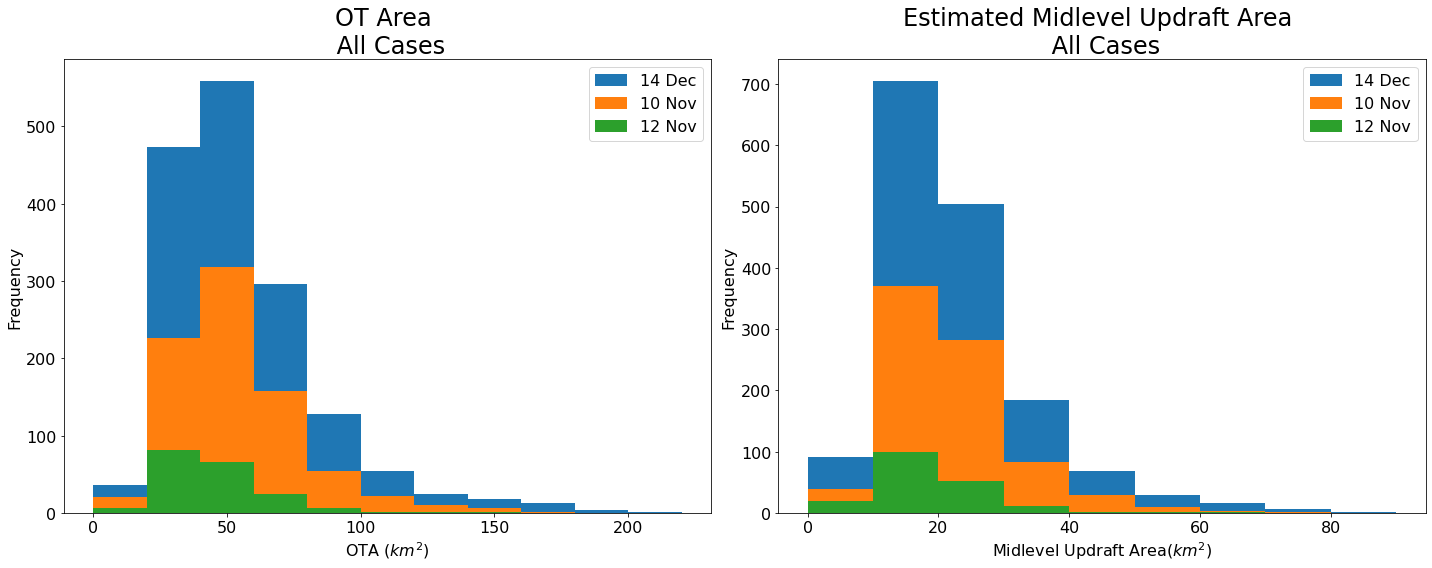
area_bins = np.arange(0, 240, 20)
ua_bins = np.arange(0, 100, 10)
fig = plt.figure(figsize=(20,8))

ax = plt.subplot(121)
ax.hist(dec_14.area_polygon, area_bins, label='14 Dec')
ax.hist(nov_10.area_polygon, area_bins, label='10 Nov')
ax.hist(nov_12.area_polygon, area_bins, label='12 Nov')


plt.title('OT Area \n All Cases', fontsize=24)

plt.xlabel('OTA ($km^2$)', fontsize=16)
plt.ylabel('Frequency', fontsize=16)

plt.xticks(fontsize=16)
plt.yticks(fontsize=16)
plt.legend(loc='upper right', fontsize=16)

ax2 = plt.subplot(122)
#plt.hist(df_max.area_polygon * 0.4032)

ax2.hist(dec_14.area_polygon * 0.4032, ua_bins, label='14 Dec')
ax2.hist(nov_10.area_polygon * 0.4032, ua_bins, label='10 Nov')
ax2.hist(nov_12.area_polygon * 0.4032, ua_bins, label='12 Nov')


plt.title('Estimated Midlevel Updraft Area \n All Cases', fontsize=24)

plt.xlabel('Midlevel Updraft Area($km^2$)', fontsize=16)
plt.ylabel('Frequency', fontsize=16)

plt.xticks(fontsize=16)
plt.yticks(fontsize=16)

plt.legend(loc='upper right', fontsize=16)

plt.tight_layout()
plt.savefig('ota_updraft_area.png', dpi=300)

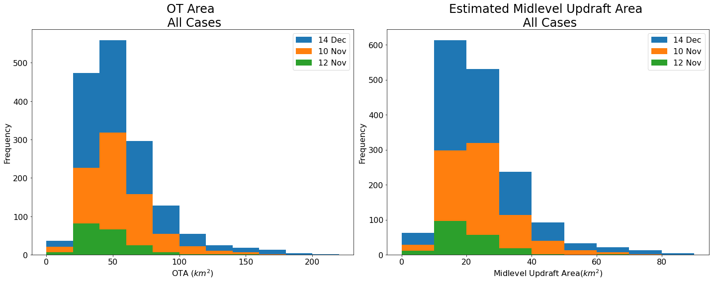
### NEW METHOD - using max ua and max ota from each case --> scaling from there (subsitute 0.44 for scaling factor now)
area_bins = np.arange(0, 240, 20)
ua_bins = np.arange(0, 100, 10)
fig = plt.figure(figsize=(20,8))

ax = plt.subplot(121)
ax.hist(dec_14.area_polygon, area_bins, label='14 Dec')
ax.hist(nov_10.area_polygon, area_bins, label='10 Nov')
ax.hist(nov_12.area_polygon, area_bins, label='12 Nov')


plt.title('OT Area \n All Cases', fontsize=24)

plt.xlabel('OTA ($km^2$)', fontsize=16)
plt.ylabel('Frequency', fontsize=16)

plt.xticks(fontsize=16)
plt.yticks(fontsize=16)
plt.legend(loc='upper right', fontsize=16)

ax2 = plt.subplot(122)
#plt.hist(df_max.area_polygon * 0.4032)

ax2.hist(dec_14.area_polygon * 0.44, ua_bins, label='14 Dec')
ax2.hist(nov_10.area_polygon * 0.44, ua_bins, label='10 Nov')
ax2.hist(nov_12.area_polygon * 0.44, ua_bins, label='12 Nov')


plt.title('Estimated Midlevel Updraft Area \n All Cases', fontsize=24)

plt.xlabel('Midlevel Updraft Area($km^2$)', fontsize=16)
plt.ylabel('Frequency', fontsize=16)

plt.xticks(fontsize=16)
plt.yticks(fontsize=16)

plt.legend(loc='upper right', fontsize=16)

plt.tight_layout()
plt.savefig('ota_updraft_area.png', dpi=300)

np.median(calc_r(df.area_polygon, 0.44))

2.5760505730140073

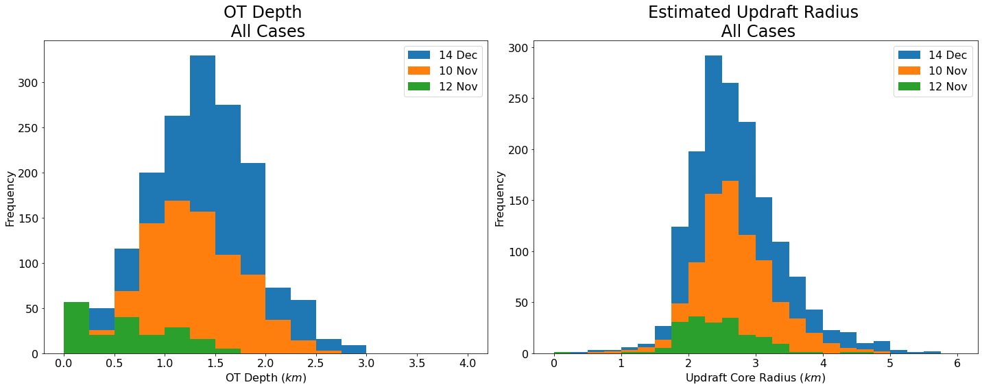
depth_bins = np.arange(0, 4.25, .25)
fig = plt.figure(figsize=(20,8))

ax = plt.subplot(121)
ax.hist(dec_14.ot_depth, depth_bins, label='14 Dec')
ax.hist(nov_10.ot_depth, depth_bins, label='10 Nov')
ax.hist(nov_12.ot_depth, depth_bins, label='12 Nov')


plt.title('OT Depth \n All Cases', fontsize=24)

plt.xlabel('OT Depth ($km$)', fontsize=16)
plt.ylabel('Frequency', fontsize=16)

plt.xticks(fontsize=16)
plt.yticks(fontsize=16)
plt.legend(loc='upper right', fontsize=16)

ax = plt.subplot(122)
ax.hist(calc_r(dec_14.area_polygon, 0.44), u_core_bins, label='14 Dec')
ax.hist(calc_r(nov_10.area_polygon, 0.44), u_core_bins, label='10 Nov')
ax.hist(calc_r(nov_12.area_polygon, 0.44), u_core_bins, label='12 Nov')


plt.title('Estimated Updraft Radius \n All Cases', fontsize=24)

plt.xlabel('Updraft Core Radius ($km$)', fontsize=16)
plt.ylabel('Frequency', fontsize=16)

plt.xticks(fontsize=16)
plt.yticks(fontsize=16)
plt.legend(loc='upper right', fontsize=16)
plt.tight_layout()
plt.savefig('ot_depth_radius', dpi=300)

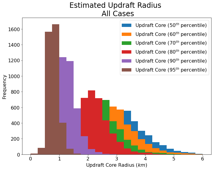
plt.figure(figsize=(10,8))
ax = plt.subplot(111)
ax.hist(df.mid_ur_50, u_core_bins, label='Updraft Core ($50^{th}$ percentile)')
ax.hist(df.mid_ur_60, u_core_bins, label='Updraft Core ($60^{th}$ percentile)')
ax.hist(df.mid_ur_70, u_core_bins, label='Updraft Core ($70^{th}$ percentile)')
ax.hist(df.mid_ur_80, u_core_bins, label='Updraft Core ($80^{th}$ percentile)')
ax.hist(df.mid_ur_90, u_core_bins, label='Updraft Core ($90^{th}$ percentile)')
ax.hist(df.mid_ur_95, u_core_bins, label='Updraft Core ($95^{th}$ percentile)')

plt.title('Estimated Updraft Radius \n All Cases', fontsize=24)

plt.xlabel('Updraft Core Radius ($km$)', fontsize=16)
plt.ylabel('Frequency', fontsize=16)

plt.xticks(fontsize=16)
plt.yticks(fontsize=16)
plt.legend(loc='upper right', fontsize=16)
plt.tight_layout()

plt.savefig('threshold_test_radii.png', dpi=300)

np.median(df.est_wmax)

41.76545649337769

np.nanpercentile(dec_14.est_wmax, 50)

47.2942793579101

np.median(df.est_wmax * 0.386)

16.121478808605172

wmax_bins = np.arange(0, 80, 10)
wmean_bins = np.arange(0,35,5)

fig = plt.figure(figsize=(20,8))

ax = plt.subplot(121)
ax.hist(dec_14.ot_depth * 22.78, wmax_bins, label='14 Dec')
ax.hist(nov_10.ot_depth * 22.78, wmax_bins, label='10 Nov')
ax.hist(nov_12.ot_depth * 22.78, wmax_bins, label='12 Nov')


plt.title('Estimated Midlevel $W_{max}$ \n All Cases', fontsize=24)

plt.xlabel('$W_{max}$ ($m/s$)', fontsize=16)
plt.ylabel('Frequency', fontsize=16)

plt.xticks(fontsize=16)
plt.yticks(fontsize=16)
plt.legend(loc='upper right', fontsize=16)


ax = plt.subplot(122)
ax.hist(dec_14.ot_depth * 8.89, wmean_bins, label='14 Dec')
ax.hist(nov_10.ot_depth * 8.89, wmean_bins, label='10 Nov')
ax.hist(nov_12.ot_depth * 8.89, wmean_bins, label='12 Nov')


plt.title('Estimated Midlevel $W_{mean}$ \n All Cases', fontsize=24)

plt.xlabel('$W_{mean}$ ($m/s$)', fontsize=16)
plt.ylabel('Frequency', fontsize=16)

plt.xticks(fontsize=16)
plt.yticks(fontsize=16)
plt.legend(loc='upper right', fontsize=16)

plt.tight_layout()
plt.savefig('Estimated_wmax_wmean.png', dpi=300)

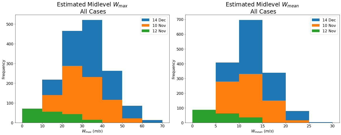
np.median(df.ot_depth * 8.89)

10.845793895721421

np.median(dec_14.est_wmax * 0.386)

18.2555918321533

np.median(df.ot_depth * wmean_scale)

10.857993888854981

wmax_scale = 22.8
wmean_scale = 8.9

wmax_bins = np.arange(0, 90, 5)
wmean_bins = np.arange(0,50,5)

fig = plt.figure(figsize=(20,8))

ax = plt.subplot(121)
ax.hist(dec_14.ot_depth * wmax_scale, wmax_bins, label='14 Dec',
        color='white', edgecolor='tab:blue', linewidth=3)
ax.hist(nov_10.ot_depth * wmax_scale, wmax_bins, label='10 Nov',
        color='white', edgecolor='tab:red', linewidth=3)
ax.hist(nov_12.ot_depth * wmax_scale, wmax_bins, label='12 Nov',
        color='white', edgecolor='tab:green', linewidth=3)


plt.title('Estimated Midlevel $W_{max}$ \n All Cases', fontsize=24)

plt.xlabel('$W_{max}$ ($ms^-1$)', fontsize=16)
plt.ylabel('Frequency', fontsize=16)

plt.xticks(fontsize=16)
plt.yticks(fontsize=16)
plt.legend(loc='upper right', fontsize=16)


ax = plt.subplot(122)
ax.hist(dec_14.ot_depth * wmean_scale, wmean_bins, label='14 Dec',
        color='white', edgecolor='tab:blue', linewidth=3)
ax.hist(nov_10.ot_depth * wmean_scale, wmean_bins, label='10 Nov',
        color='white', edgecolor='tab:red', linewidth=3)
ax.hist(nov_12.ot_depth * wmean_scale, wmean_bins, label='12 Nov',
        color='white', edgecolor='tab:green', linewidth=3)


plt.title('Estimated Midlevel $W_{mean}$ \n All Cases', fontsize=24)

plt.xlabel('$W_{mean}$ ($ms^-1$)', fontsize=16)
plt.ylabel('Frequency', fontsize=16)

plt.xticks(fontsize=16)
plt.yticks(fontsize=16)
plt.legend(loc='upper right', fontsize=16)

plt.tight_layout()
plt.savefig('Estimated_wmax_wmean.png', dpi=300)

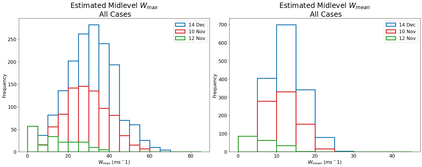
np.max(df.ot_depth * wmax_scale)

71.16473251342774

np.sqrt(2 * 2900)

76.15773105863909

u_core_bins = np.arange(0, 6.25, .25)
ua_bins = np.arange(0, 100, 10)
fig = plt.figure(figsize=(20,8))

ax = plt.subplot(121)
ax.hist(calc_r(dec_14.area_polygon), u_core_bins, label='14 Dec')
ax.hist(calc_r(nov_10.area_polygon), u_core_bins, label='10 Nov')
ax.hist(calc_r(nov_12.area_polygon), u_core_bins, label='12 Nov')


plt.title('Estimated Updraft Radius \n All Cases', fontsize=24)

plt.xlabel('Updraft Core Radius ($km$)', fontsize=16)
plt.ylabel('Frequency', fontsize=16)

plt.xticks(fontsize=16)
plt.yticks(fontsize=16)
plt.legend(loc='upper right', fontsize=16)

ax2 = plt.subplot(122)
#plt.hist(df_max.area_polygon * 0.4032)



ax2.hist(dec_14.area_polygon * 0.4032, ua_bins, label='14 Dec')
ax2.hist(nov_10.area_polygon * 0.4032, ua_bins, label='10 Nov')
ax2.hist(nov_12.area_polygon * 0.4032, ua_bins, label='12 Nov')


plt.title('Estimated Updraft Area \n All Cases', fontsize=24)

plt.xlabel('Updraft Core Area($km^2$)', fontsize=16)
plt.ylabel('Frequency', fontsize=16)

plt.xticks(fontsize=16)
plt.yticks(fontsize=16)

plt.legend(loc='upper right', fontsize=16)

plt.savefig('Updraft_Radius_Area.png', dpi=400)

wmax_bins = np.arange(0, 105, 5)
df.est_wmax.plot.hist(bins=wmax_bins)

<AxesSubplot:ylabel='Frequency'>

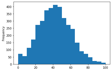
plt.figure(figsize=(10,8))
bins = np.arange(0, 10.25, .25)
df.mid_ud.plot.hist(bins=bins)

<AxesSubplot:ylabel='Frequency'>

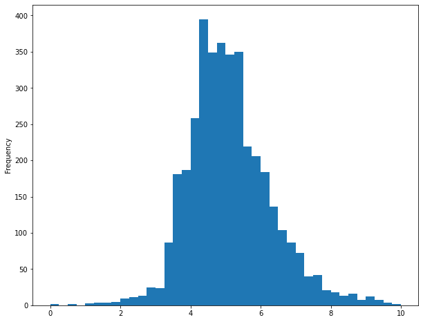
df['est_wmax'] = df.ot_depth * 34.238

/data/keeling/a/mgrover4/a/miniconda3/envs/xesmf_env/lib/python3.7/site-packages/ipykernel_launcher.py:1: SettingWithCopyWarning: 
A value is trying to be set on a copy of a slice from a DataFrame.
Try using .loc[row_indexer,col_indexer] = value instead

See the caveats in the documentation: https://pandas.pydata.org/pandas-docs/stable/user_guide/indexing.html#returning-a-view-versus-a-copy
  """Entry point for launching an IPython kernel.

df.est_wmax.plot.hist()

<AxesSubplot:ylabel='Frequency'>

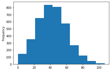
df['lat_rounded'] = np.round(df.lat, 0)
df['lon_rounded'] = np.round(df.lon, 0)

/data/keeling/a/mgrover4/a/miniconda3/envs/xesmf_env/lib/python3.7/site-packages/ipykernel_launcher.py:1: SettingWithCopyWarning: 
A value is trying to be set on a copy of a slice from a DataFrame.
Try using .loc[row_indexer,col_indexer] = value instead

See the caveats in the documentation: https://pandas.pydata.org/pandas-docs/stable/user_guide/indexing.html#returning-a-view-versus-a-copy
  """Entry point for launching an IPython kernel.
/data/keeling/a/mgrover4/a/miniconda3/envs/xesmf_env/lib/python3.7/site-packages/ipykernel_launcher.py:2: SettingWithCopyWarning: 
A value is trying to be set on a copy of a slice from a DataFrame.
Try using .loc[row_indexer,col_indexer] = value instead

See the caveats in the documentation: https://pandas.pydata.org/pandas-docs/stable/user_guide/indexing.html#returning-a-view-versus-a-copy
  

nov_10_all = df[df.day == 10]
nov_12_all = df[df.day == 12]
dec_14_all = df[df.day == 14]

u_core_bins * 2

---------------------------------------------------------------------------
NameError                                 Traceback (most recent call last)
<ipython-input-23-2dd16c05d398> in <module>
----> 1 u_core_bins * 2

NameError: name 'u_core_bins' is not defined

ur = calc_r(nov_10_all.area_polygon)
med = np.median(ur) * 2
top_perc = np.percentile(ur, 95) * 2

fig = plt.figure(figsize=(12,8))
plt.hist(ur * 2, u_core_bins * 2)

plt.axvline(med, color='r', linewidth=3, label=f'Median: {np.round(med,2)} km')
plt.axvline(top_perc, color='b', linewidth=3, label='$95^{th}$' + f' Perc: {np.round(top_perc, 2)} km')

plt.title('OTA Distribution \n All OTs', fontsize=24)

plt.xlabel('Updraft Core Radius ($km$)', fontsize=16)
plt.ylabel('Frequency', fontsize=16)
plt.xticks(fontsize=14)
plt.yticks(fontsize=14)
plt.legend(fontsize=16)

<matplotlib.legend.Legend at 0x2af2f3d18f60>

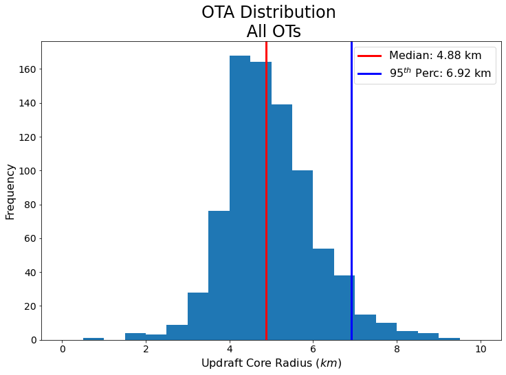
ur = calc_r(nov_12_all.area_polygon)
med = np.median(ur) * 2
top_perc = np.percentile(ur, 95) * 2

fig = plt.figure(figsize=(12,8))
plt.hist(ur * 2, u_core_bins * 2)

plt.axvline(med, color='r', linewidth=3, label=f'Median: {np.round(med,2)} km')
plt.axvline(top_perc, color='b', linewidth=3, label='$95^{th}$' + f' Perc: {np.round(top_perc, 2)} km')

plt.title('OTA Distribution \n All OTs', fontsize=24)

plt.xlabel('Updraft Core Radius ($km$)', fontsize=16)
plt.ylabel('Frequency', fontsize=16)

plt.xticks(fontsize=14)
plt.yticks(fontsize=14)
plt.legend(fontsize=16)

<matplotlib.legend.Legend at 0x2af2f3d4b208>

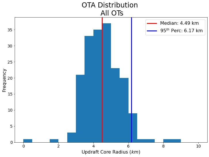
ur = calc_r(dec_14_all.area_polygon)
med = np.median(ur) * 2
top_perc = np.percentile(ur, 95) * 2

fig = plt.figure(figsize=(12,8))
plt.hist(ur * 2, u_core_bins * 2)

plt.axvline(med, color='r', linewidth=3, label=f'Median: {np.round(med,2)} km')
plt.axvline(top_perc, color='b', linewidth=3, label='$95^{th}$' + f' Perc: {np.round(top_perc, 2)} km')

plt.title('OTA Distribution \n All OTs', fontsize=24)

plt.xlabel('Updraft Core Radius ($km$)', fontsize=16)
plt.ylabel('Frequency', fontsize=16)

plt.xticks(fontsize=14)
plt.yticks(fontsize=14)
plt.legend(fontsize=16)

<matplotlib.legend.Legend at 0x2af2f3d8d978>

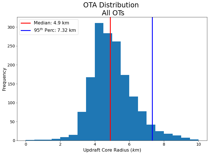
llcrnr=[-33.206342, -65.906586]
urcrnr=[-30.255825, -62.630553]

# Set extent of maps created in the following cells:
axis_extent=[llcrnr[1],urcrnr[1],llcrnr[0],urcrnr[0]]    

# Plot map with all individual tracks:
import cartopy.crs as ccrs
fig_map,ax_map=plt.subplots(figsize=(15,15),subplot_kw={'projection': ccrs.PlateCarree()})

ax_map.coastlines()

ax_map.set_extent(axis_extent)

for ds in ds_list:
#    cm = ax.contourf(ds.x.values[::5], ds.y.values[::5], ds.values[::5,::5], levs, cmap='terrain', transform=ccrs.PlateCarree())
    cm = ax_map.imshow(ds.values, extent =[ds.x.min(),ds.x.max(),ds.y.min(),ds.y.max()], transform=ccrs.PlateCarree(), vmin=0, vmax=4000, cmap='terrain')

gl = ax_map.gridlines(crs=ccrs.PlateCarree(), draw_labels=True,
                  linewidth=2, color='gray', alpha=0.5, linestyle='--')

#for name, group in cells_grouped:
#    print(group.x,group.y)
#    cm2 = plt.scatter(group.lon,group.lat,c=group.area_polygon,vmin=0.,vmax=200.,s=group.area_polygon,
#                     facecolors='none',cmap='magma',linewidth=0.5)

#plt.colorbar(cm,label='Elevation (m)',shrink=0.4, pad=0.0)
#plt.colorbar(cm2,label='OT Area (km$^2$)',shrink=0.4, pad=0.1)

ax.add_feature(cfeature.STATES, linestyle=":")

plt.axvline(-65, linewidth=3)
plt.axhline(-32, linewidth=3)


ax_map.set_title('Overshooting top tracks\n14 December 2018')

Text(0.5, 1.0, 'Overshooting top tracks\n14 December 2018')

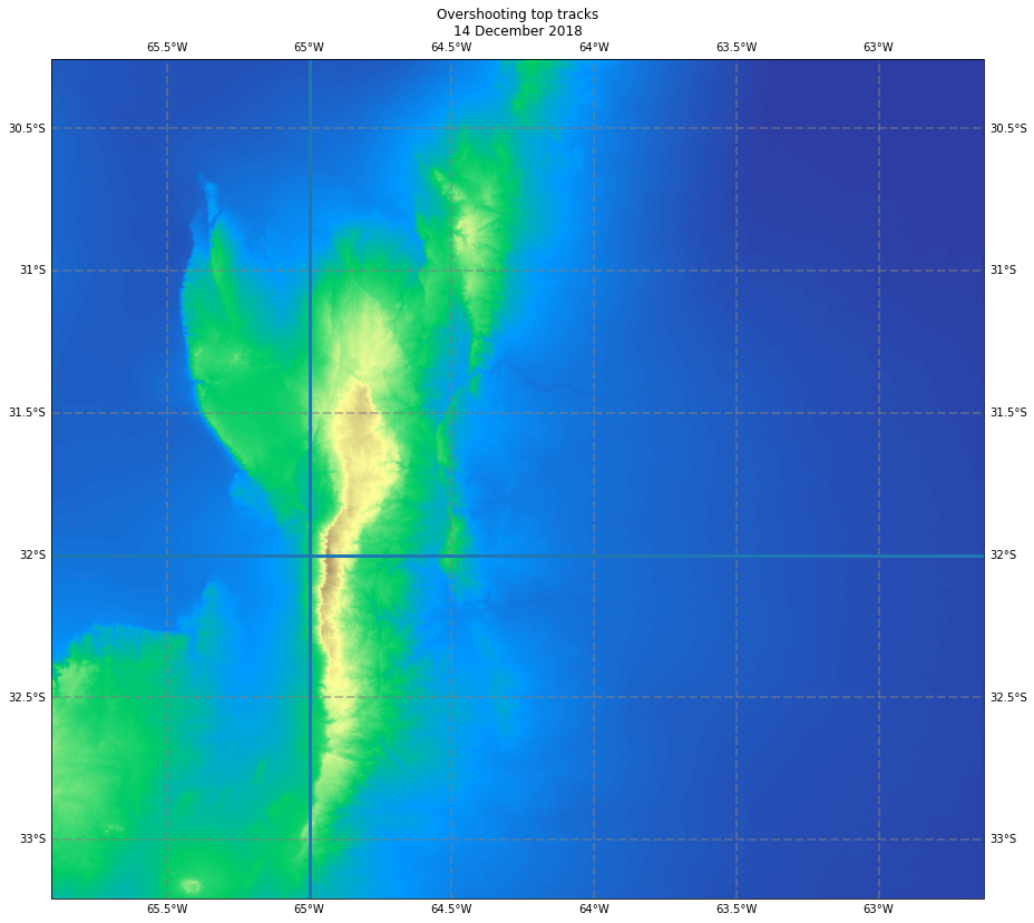
fig = plt.figure(figsize=(12,8))
plt.hist(df.area_polygon, bins=ota_bins)

plt.title('OTA Distribution \n All OTs', fontsize=24)

plt.xlabel('OTA ($km^2$)', fontsize=16)
plt.ylabel('Frequency', fontsize=16)

Text(0, 0.5, 'Frequency')

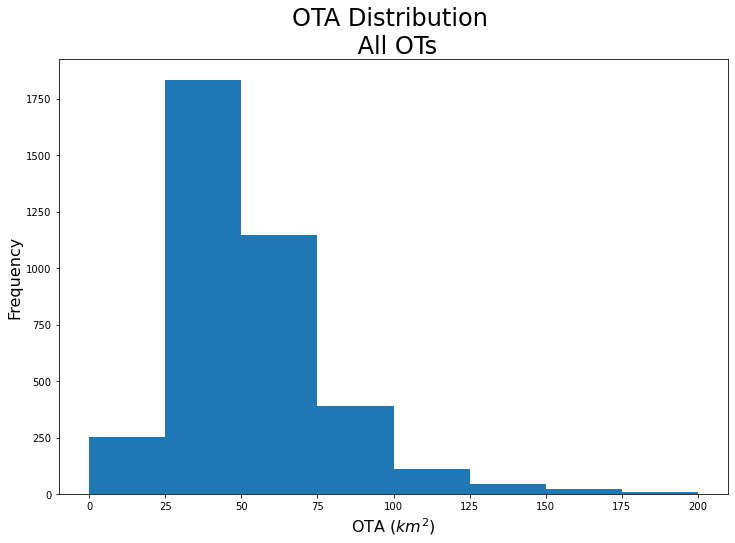
u_core_bins = np.arange(0, 5.25, .25)

np.median(calc_r(df_max.area_polygon)) * 2

5.498395714122815

np.median(calc_r(df.area_polygon)) * 2

4.769737992345483

hist, bins = np.histogram(calc_r(df.area_polygon), bins=10, normed=True)
bin_centers = (bins[1:]+bins[:-1])*0.5
plt.bar(bin_centers, hist)

/data/keeling/a/mgrover4/a/miniconda3/envs/xesmf_env/lib/python3.7/site-packages/ipykernel_launcher.py:1: VisibleDeprecationWarning: Passing `normed=True` on non-uniform bins has always been broken, and computes neither the probability density function nor the probability mass function. The result is only correct if the bins are uniform, when density=True will produce the same result anyway. The argument will be removed in a future version of numpy.
  """Entry point for launching an IPython kernel.

<BarContainer object of 10 artists>

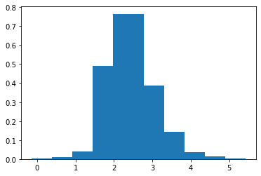
fig = plt.figure(figsize=(12,8))
plt.hist(calc_r(df.area_polygon), u_core_bins)

plt.title('OTA Distribution \n All OTs', fontsize=24)

plt.xlabel('Updraft Core Radius ($km$)', fontsize=16)
plt.ylabel('Frequency', fontsize=16)

Text(0, 0.5, 'Frequency')

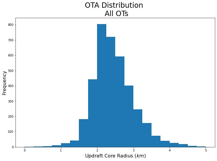
fig = plt.figure(figsize=(12,8))
plt.hist(calc_r(nov_10.area_polygon), u_core_bins)

plt.title('OTA Distribution \n All OTs', fontsize=24)

plt.xlabel('Updraft Core Radius ($km$)', fontsize=16)
plt.ylabel('Frequency', fontsize=16)

Text(0, 0.5, 'Frequency')

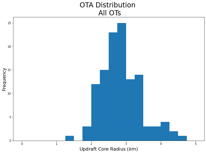
fig = plt.figure(figsize=(12,8))
plt.hist(df_max.area_polygon * 0.4032)

plt.title('Updraft Area Distribution \n All OTs', fontsize=24)

plt.xlabel('Updraft Core Area($km^2$)', fontsize=16)
plt.ylabel('Frequency', fontsize=16)

Text(0, 0.5, 'Frequency')

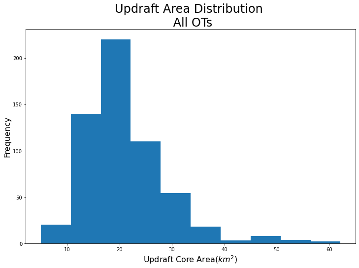
fig = plt.figure(figsize=(12,8))
plt.hist(df_max.area_polygon)

plt.title('OTA Distribution \n All OTs', fontsize=24)

plt.xlabel('OTA ($km^2$)', fontsize=16)
plt.ylabel('Frequency', fontsize=16)

Text(0, 0.5, 'Frequency')

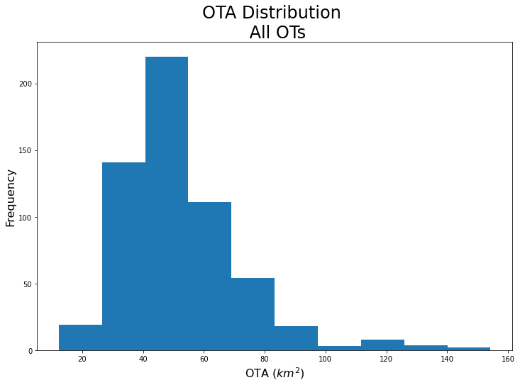
slope, intercept, r, p, stderr = scipy.stats.linregress(df_max.mid_ur, df_max.ot_depth)

line = f'r={r:.2f}'

plt.figure(figsize=(10,8))
ax = plt.subplot(111)
#max_depth_nov_10 = max_depth[max_depth.day == 10]
ax.scatter(dec_14.mid_ur, dec_14.ot_depth, color='tab:blue', label='14 December 2018')
ax.scatter(nov_12.mid_ur, nov_12.ot_depth, color='tab:green', label='12 November 2018')
ax.scatter(nov_10.mid_ur, nov_10.ot_depth, color='tab:red', label='10 November 2018')

ax.scatter(np.median(dec_14.mid_ur), np.median(dec_14.ot_depth), color='blue', s=100)
ax.scatter(np.median(nov_10.mid_ur), np.median(nov_10.ot_depth), color='red', s=100)
ax.scatter(np.median(nov_12.mid_ur), np.median(nov_12.ot_depth), color='green', s=100)

ax.plot(np.array(df_max.mid_ur), intercept + slope * np.array(df_max.mid_ur), label=line, color='black')

plt.xlabel('Midlevel Updraft Radius ($km$)', fontsize=12)
plt.ylabel('OT Depth $(km)$', fontsize=12)

plt.legend(loc='upper right', fontsize=12)

plt.title('OT Duration All OTs  \n 10 November, 12 November, 14 December 2018 UTC (Count = 1022)', fontsize=16)

---------------------------------------------------------------------------
AttributeError                            Traceback (most recent call last)
<ipython-input-102-decea871942b> in <module>
----> 1 slope, intercept, r, p, stderr = scipy.stats.linregress(df_max.mid_ur, df_max.ot_depth)
      2 
      3 line = f'r={r:.2f}'
      4 
      5 plt.figure(figsize=(10,8))

~/a/miniconda3/envs/xesmf_env/lib/python3.7/site-packages/pandas/core/generic.py in __getattr__(self, name)
   5139             if self._info_axis._can_hold_identifiers_and_holds_name(name):
   5140                 return self[name]
-> 5141             return object.__getattribute__(self, name)
   5142 
   5143     def __setattr__(self, name: str, value) -> None:

AttributeError: 'DataFrame' object has no attribute 'mid_ur'

plt.figure(figsize=(10,8))
ax = plt.subplot(111)
#max_depth_nov_10 = max_depth[max_depth.day == 10]
ax.scatter(dec_14.mid_ur, dec_14.duration, color='tab:blue', label='14 December 2018')
ax.scatter(nov_12.mid_ur, nov_12.duration, color='tab:green', label='12 November 2018')
ax.scatter(nov_10.mid_ur, nov_10.duration, color='tab:red', label='10 November 2018')

ax.scatter(np.mean(dec_14.mid_ur), np.mean(dec_14.duration), color='blue', s=100)
ax.scatter(np.mean(nov_10.mid_ur), np.mean(nov_10.duration), color='red', s=100)
ax.scatter(np.mean(nov_12.mid_ur), np.mean(nov_12.duration), color='green', s=100)

#ax.plot(np.array(df_max.mid_ur), intercept + slope * np.array(df_max.mid_ur), label=line, color='black')

plt.xlabel('Estimated Midlevel \n Updraft Radius ($km$)', fontsize=12)
plt.ylabel('OT Duration $(km)$', fontsize=12)

plt.legend(loc='upper right', fontsize=12)

plt.xlim(0,5)
plt.ylim(2,16)

plt.title('OT Duration All OTs  \n 10 November, 12 November, 14 December 2018 UTC (Count = 1022)', fontsize=16)

Text(0.5, 1.0, 'OT Duration All OTs  \n 10 November, 12 November, 14 December 2018 UTC (Count = 1022)')

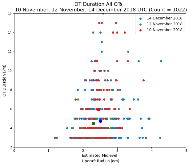
plt.scatter(df_max.ot_depth, df_max.mid_ur)

<matplotlib.collections.PathCollection at 0x2b5e68d12cf8>

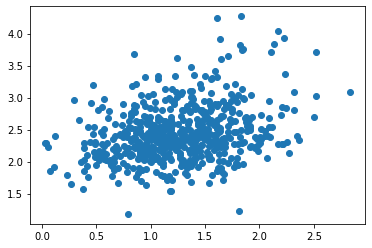
uar_dec14 = calc_r(dec_14.area_polygon)
uar_nov10 = calc_r(nov_10.area_polygon)
uar_nov12 = calc_r(nov_10.area_polygon)

ota = df_max.area_polygon
u_r = calc_r(ota)
ot_r = calc_r(ota, 1)

np.percentile(u_r, 90)

3.0136419031378203

slope, intercept, r, p, stderr = scipy.stats.linregress(u_r, df_max.ot_depth)

df_max['u_diam'] = np.round(u_r* 2, 0)
df_max['round_area'] = np.round(df_max.area_polygon, -1)

fig = plt.figure(figsize=(12,8))

ax = plt.subplot(111)
df_max.boxplot('ot_depth', by='u_diam', ax=ax)

<AxesSubplot:title={'center':'ot_depth'}, xlabel='u_diam'>

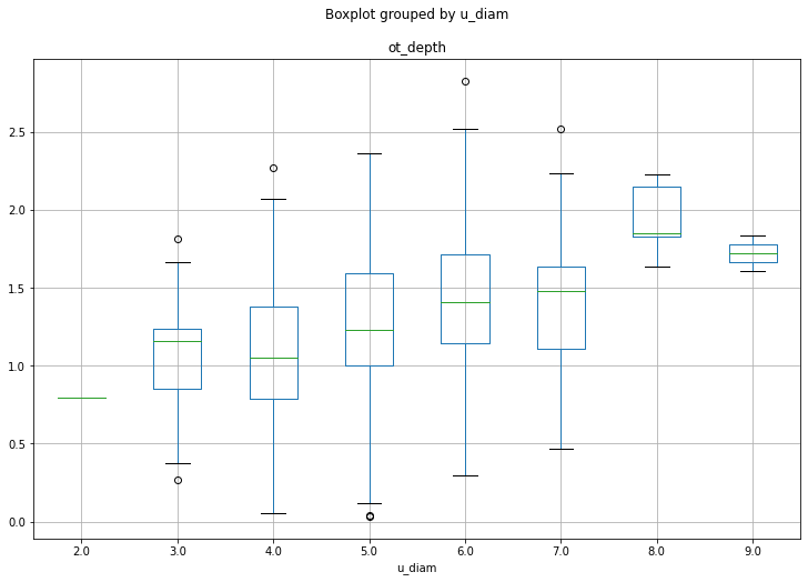
plt.scatter(u_r, df_max.ot_depth)

<matplotlib.collections.PathCollection at 0x2b56fb31a240>

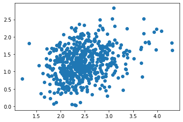
np.median(calc_r(dec_14.area_polygon)) * 2

4.894120115882311

np.median(calc_r(dec_14.area_polygon))

2.4470600579411554

mean_nov10 = np.mean(calc_r(nov_10.area_polygon) * 2)
mean_nov12 = np.mean(calc_r(nov_12.area_polygon) * 2)
mean_dec14 = np.mean(calc_r(dec_14.area_polygon) * 2)

std_nov10 = np.std(calc_r(nov_10.area_polygon) * 2)
std_nov12 = np.std(calc_r(nov_12.area_polygon) * 2)
std_dec14 = np.std(calc_r(dec_14.area_polygon) * 2)

plt.bar('Nov 10', mean_nov10)
plt.bar('Nov 12', mean_nov12)
plt.bar('Dec 14', mean_nov12)



plt.ylim(4,6)

(4.0, 6.0)

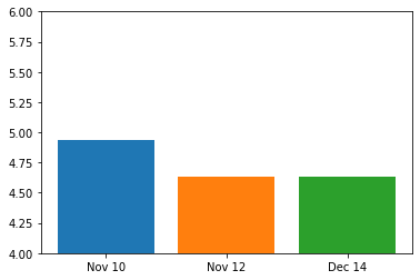
plt.hist(calc_r(nov_12.area_polygon), u_core_bins, label='12 Nov')

(array([0., 0., 0., 0., 0., 0., 2., 6., 4., 7., 3., 5., 0., 0., 0., 0., 0.,
        0., 0., 0.]),
 array([0.  , 0.25, 0.5 , 0.75, 1.  , 1.25, 1.5 , 1.75, 2.  , 2.25, 2.5 ,
        2.75, 3.  , 3.25, 3.5 , 3.75, 4.  , 4.25, 4.5 , 4.75, 5.  ]),
 <BarContainer object of 20 artists>)

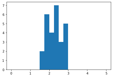
plt.hist(calc_r(nov_10.area_polygon), u_core_bins, label='12 Nov')

(array([ 0.,  0.,  0.,  0.,  1.,  0.,  1., 11., 19., 35., 28., 10., 10.,
         3.,  0.,  1.,  0.,  0.,  0.,  0.]),
 array([0.  , 0.25, 0.5 , 0.75, 1.  , 1.25, 1.5 , 1.75, 2.  , 2.25, 2.5 ,
        2.75, 3.  , 3.25, 3.5 , 3.75, 4.  , 4.25, 4.5 , 4.75, 5.  ]),
 <BarContainer object of 20 artists>)

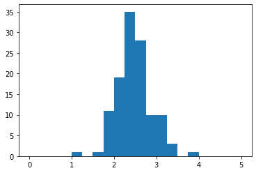
plt.hist(calc_r(dec_14.area_polygon), u_core_bins, label='14 Dec')

(array([ 0.,  0.,  0.,  0.,  0.,  1.,  5., 22., 42., 68., 49., 35., 15.,
         7.,  6.,  5.,  0.,  2.,  0.,  0.]),
 array([0.  , 0.25, 0.5 , 0.75, 1.  , 1.25, 1.5 , 1.75, 2.  , 2.25, 2.5 ,
        2.75, 3.  , 3.25, 3.5 , 3.75, 4.  , 4.25, 4.5 , 4.75, 5.  ]),
 <BarContainer object of 20 artists>)

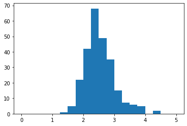
ot_core_bins = np.arange(0, 10, .25)

fig = plt.figure(figsize=(20,8))

ax = plt.subplot(121)
ax.hist(calc_r(dec_14.area_polygon, 1), ot_core_bins, label='14 Dec')
ax.hist(calc_r(nov_10.area_polygon, 1), ot_core_bins, label='10 Nov')
ax.hist(calc_r(nov_12.area_polygon, 1), ot_core_bins, label='12 Nov')


plt.title('OT Effective Radius \n All Cases', fontsize=24)

plt.xlabel('OT Radius ($km$)', fontsize=16)
plt.ylabel('Frequency', fontsize=16)

plt.xticks(fontsize=16)
plt.yticks(fontsize=16)
plt.legend(loc='upper right', fontsize=16)

ax2 = plt.subplot(122)
#plt.hist(df_max.area_polygon * 0.4032)



ax2.hist(dec_14.area_polygon, bins=ota_bins, label='14 Dec')
ax2.hist(nov_10.area_polygon, bins=ota_bins, label='10 Nov')
ax2.hist(nov_12.area_polygon, bins=ota_bins, label='12 Nov')


plt.title('OTA \n All Cases', fontsize=24)

plt.xlabel('OTA ($km^2$)', fontsize=16)
plt.ylabel('Frequency', fontsize=16)

plt.xticks(fontsize=16)
plt.yticks(fontsize=16)

plt.legend(loc='upper right', fontsize=16)

plt.savefig('OT_Radius_Duration.png', dpi=400)

---------------------------------------------------------------------------
NameError                                 Traceback (most recent call last)
<ipython-input-33-25ad375b8cf8> in <module>
      2 
      3 ax = plt.subplot(121)
----> 4 ax.hist(calc_r(dec_14.area_polygon, 1), ot_core_bins, label='14 Dec')
      5 ax.hist(calc_r(nov_10.area_polygon, 1), ot_core_bins, label='10 Nov')
      6 ax.hist(calc_r(nov_12.area_polygon, 1), ot_core_bins, label='12 Nov')

NameError: name 'ot_core_bins' is not defined

fig = plt.figure(figsize=(20,8))

ax = plt.subplot(121)
ax.hist(calc_r(df_max.area_polygon, 1), ot_core_bins, label='14 Dec')


plt.title('OT Effective Radius \n All Cases', fontsize=24)

plt.xlabel('OT Radius ($km$)', fontsize=16)
plt.ylabel('Frequency', fontsize=16)

plt.xticks(fontsize=16)
plt.yticks(fontsize=16)
#plt.legend(loc='upper right', fontsize=16)

ax2 = plt.subplot(122)
#plt.hist(df_max.area_polygon * 0.4032)



ax2.hist(df_max.area_polygon, bins=ota_bins, label='14 Dec')


plt.title('OTA \n All Cases', fontsize=24)

plt.xlabel('OTA ($km^2$)', fontsize=16)
plt.ylabel('Frequency', fontsize=16)

plt.xticks(fontsize=16)
plt.yticks(fontsize=16)

#plt.legend(loc='upper right', fontsize=16)

plt.savefig('OT_Radius_Duration.png', dpi=400)

---------------------------------------------------------------------------
NameError                                 Traceback (most recent call last)
<ipython-input-14-d85d0451eb01> in <module>
      2 
      3 ax = plt.subplot(121)
----> 4 ax.hist(calc_r(df_max.area_polygon, 1), ot_core_bins, label='14 Dec')
      5 
      6 

NameError: name 'calc_r' is not defined

nov_10 = df[df.day == 10]
nov_12 = df[df.day == 12]
dec_14 = df[df.day == 14]

nov_10_mean = nov_10.groupby('cell').mean()
nov_12_mean = nov_12.groupby('cell').mean()
dec_14_mean = dec_14.groupby('cell').mean()

nov_10_max = nov_10.groupby('cell').max()
nov_12_max = nov_12.groupby('cell').max()
dec_14_max = dec_14.groupby('cell').max()

u_core_bins = np.arange(0, 6.25, .25)
ua_bins = np.arange(0, 100, 10)
fig = plt.figure(figsize=(20,8))

ax = plt.subplot(121)
ax.hist(calc_r(dec_14.area_polygon), u_core_bins, label='14 Dec')
ax.hist(calc_r(nov_10.area_polygon), u_core_bins, label='10 Nov')
ax.hist(calc_r(nov_12.area_polygon), u_core_bins, label='12 Nov')


plt.title('Estimated Updraft Radius \n All Cases', fontsize=24)

plt.xlabel('Updraft Core Radius ($km$)', fontsize=16)
plt.ylabel('Frequency', fontsize=16)

plt.xticks(fontsize=16)
plt.yticks(fontsize=16)
plt.legend(loc='upper right', fontsize=16)

ax2 = plt.subplot(122)
#plt.hist(df_max.area_polygon * 0.4032)



ax2.hist(dec_14.area_polygon * 0.4032, ua_bins, label='14 Dec')
ax2.hist(nov_10.area_polygon * 0.4032, ua_bins, label='10 Nov')
ax2.hist(nov_12.area_polygon * 0.4032, ua_bins, label='12 Nov')


plt.title('Estimated Updraft Area \n All Cases', fontsize=24)

plt.xlabel('Updraft Core Area($km^2$)', fontsize=16)
plt.ylabel('Frequency', fontsize=16)

plt.xticks(fontsize=16)
plt.yticks(fontsize=16)

plt.legend(loc='upper right', fontsize=16)

plt.savefig('Updraft_Radius_Area.png', dpi=400)

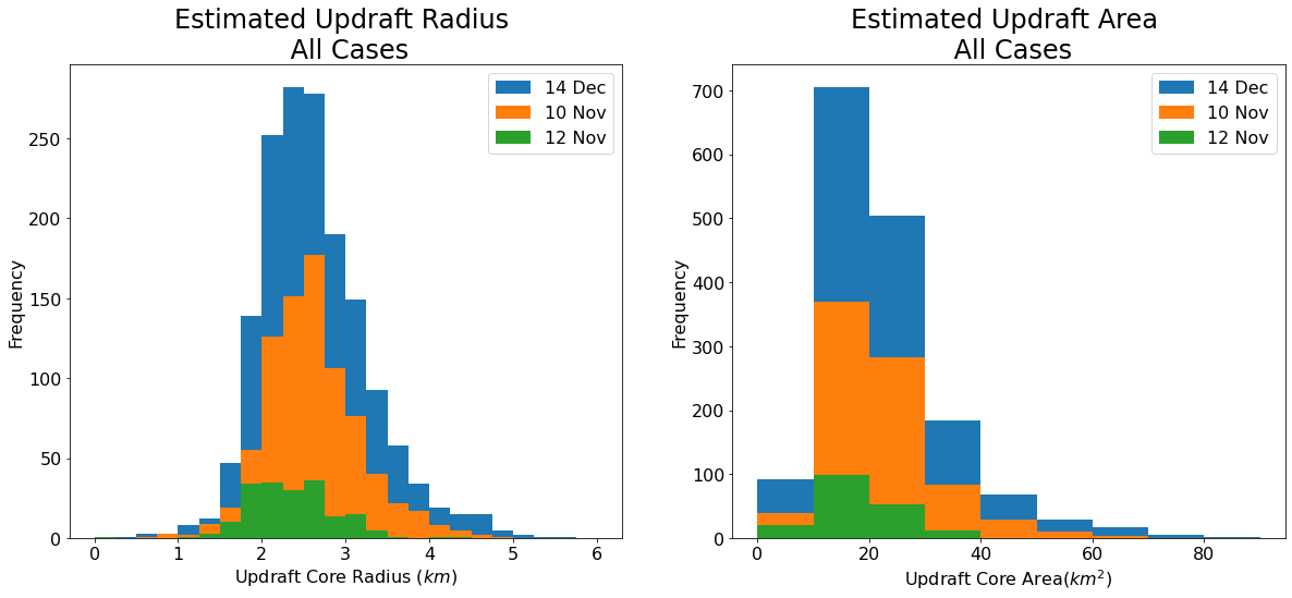
u_core_bins = np.arange(0, 6.25, .25)
ua_bins = np.arange(0, 100, 10)
fig = plt.figure(figsize=(20,8))

ax = plt.subplot(121)
ax.hist(calc_r(dec_14_mean.area_polygon), u_core_bins, label='14 Dec')
ax.hist(calc_r(nov_10_mean.area_polygon), u_core_bins, label='10 Nov')
ax.hist(calc_r(nov_12_mean.area_polygon), u_core_bins, label='12 Nov')


plt.title('Estimated Mean Updraft Radius \n All Cases', fontsize=24)

plt.xlabel('Updraft Core Radius ($km$)', fontsize=16)
plt.ylabel('Frequency', fontsize=16)

plt.xticks(fontsize=16)
plt.yticks(fontsize=16)
plt.legend(loc='upper right', fontsize=16)

ax2 = plt.subplot(122)
#plt.hist(df_max.area_polygon * 0.4032)



ax2.hist(dec_14_mean.area_polygon * 0.4032, ua_bins, label='14 Dec')
ax2.hist(nov_10_mean.area_polygon * 0.4032, ua_bins, label='10 Nov')
ax2.hist(nov_12_mean.area_polygon * 0.4032, ua_bins, label='12 Nov')


plt.title('Estimated Mean Updraft Area \n All Cases', fontsize=24)

plt.xlabel('Updraft Core Area($km^2$)', fontsize=16)
plt.ylabel('Frequency', fontsize=16)

plt.xticks(fontsize=16)
plt.yticks(fontsize=16)

plt.legend(loc='upper right', fontsize=16)

plt.savefig('Updraft_Radius_Area_mean.png', dpi=400)

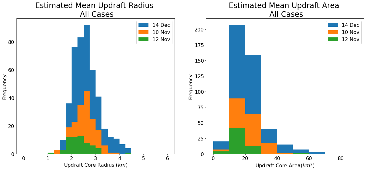
u_core_bins = np.arange(0, 6.25, .25)
ua_bins = np.arange(0, 100, 10)
fig = plt.figure(figsize=(20,8))

ax = plt.subplot(121)
ax.hist(calc_r(dec_14_max.area_polygon), u_core_bins, label='14 Dec')
ax.hist(calc_r(nov_10_max.area_polygon), u_core_bins, label='10 Nov')
ax.hist(calc_r(nov_12_max.area_polygon), u_core_bins, label='12 Nov')


plt.title('Estimated Peak Updraft Radius \n All Cases', fontsize=24)

plt.xlabel('Updraft Core Radius ($km$)', fontsize=16)
plt.ylabel('Frequency', fontsize=16)

plt.xticks(fontsize=16)
plt.yticks(fontsize=16)
plt.legend(loc='upper right', fontsize=16)

ax2 = plt.subplot(122)
#plt.hist(df_max.area_polygon * 0.4032)



ax2.hist(dec_14_max.area_polygon * 0.4032, ua_bins, label='14 Dec')
ax2.hist(nov_10_max.area_polygon * 0.4032, ua_bins, label='10 Nov')
ax2.hist(nov_12_max.area_polygon * 0.4032, ua_bins, label='12 Nov')


plt.title('Estimated Peak Updraft Area \n All Cases', fontsize=24)

plt.xlabel('Updraft Core Area($km^2$)', fontsize=16)
plt.ylabel('Frequency', fontsize=16)

plt.xticks(fontsize=16)
plt.yticks(fontsize=16)

plt.legend(loc='upper right', fontsize=16)

plt.savefig('Updraft_Radius_Area_max.png', dpi=400)

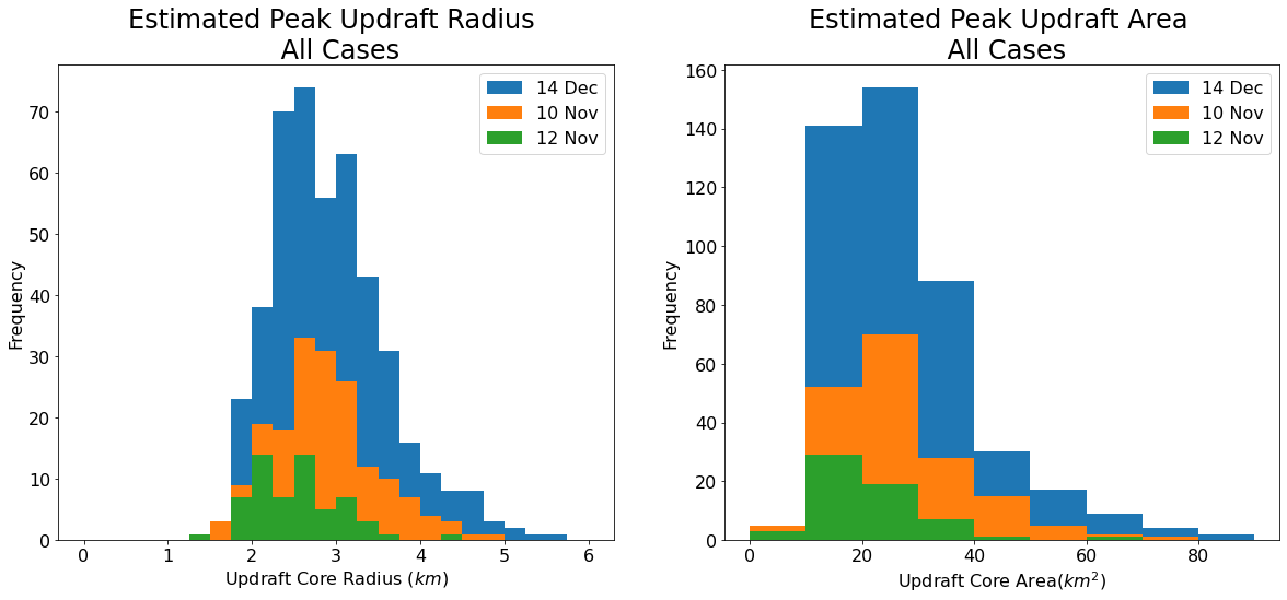
u_core_bins = np.arange(0, 6.25, .25)
ua_bins = np.arange(0, 90, 10)
fig = plt.figure(figsize=(20,8))

ax = plt.subplot(121)
ax.hist(calc_r(dec_14.area_polygon, u_core_bins, label='14 Dec')
ax.hist(nov_10.area_polygon, u_core_bins, label='10 Nov')
ax.hist(nov_12.area_polygon, u_core_bins, label='12 Nov')


plt.title('OT Radius \n All Cases', fontsize=24)

plt.xlabel('OT Radius ($km$)', fontsize=16)
plt.ylabel('Frequency', fontsize=16)

plt.xticks(fontsize=16)
plt.yticks(fontsize=16)
plt.legend(loc='upper right', fontsize=16)

ax2 = plt.subplot(122)
#plt.hist(df_max.area_polygon * 0.4032)



ax2.hist(dec_14.area_polygon, ua_bins, label='14 Dec')
ax2.hist(nov_10.area_polygon, ua_bins, label='10 Nov')
ax2.hist(nov_12.area_polygon, ua_bins, label='12 Nov')


plt.title('OT Area \n All Cases', fontsize=24)

plt.xlabel('OTA ($km^2$)', fontsize=16)
plt.ylabel('Frequency', fontsize=16)

plt.xticks(fontsize=16)
plt.yticks(fontsize=16)

plt.legend(loc='upper right', fontsize=16)

plt.savefig('OT_r_OTA_Duration.png', dpi=400)

cell
963     1.841556
971     1.036429
974     1.212000
975     1.747834
977     1.369286
          ...   
1937    0.566249
1940    0.558000
1941    1.128167
1946    1.026000
1949    0.437749
Name: ot_depth, Length: 257, dtype: float64

fig = plt.figure(figsize=(20,8))

ax = plt.subplot(121)
ax.hist(dec_14.duration, dur_bins, label='14 Dec')
ax.hist(nov_10.duration, dur_bins, label='10 Nov')
ax.hist(nov_12.duration, dur_bins, label='12 Nov')


plt.title('OT Duration \n All Cases', fontsize=24)

plt.xlabel('Duration ($min$)', fontsize=16)
plt.ylabel('Frequency', fontsize=16)

plt.xticks(fontsize=16)
plt.yticks(fontsize=16)
plt.legend(loc='upper right', fontsize=16)

ax2 = plt.subplot(122)
#plt.hist(df_max.area_polygon * 0.4032)



ax2.hist(dec_14.ot_depth, otd_bins, label='14 Dec')
ax2.hist(nov_10.ot_depth, otd_bins, label='10 Nov')
ax2.hist(nov_12.ot_depth, otd_bins, label='12 Nov')


plt.title('OT Depth \n All Cases', fontsize=24)

plt.xlabel('OT Depth ($km$)', fontsize=16)
plt.ylabel('Frequency', fontsize=16)

plt.xticks(fontsize=16)
plt.yticks(fontsize=16)

plt.legend(loc='upper right', fontsize=16)

plt.savefig('OT_Duration_OT_Depth.png', dpi=400)

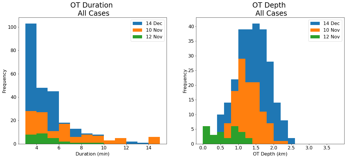
fig = plt.figure(figsize=(20,8))

ax = plt.subplot(121)
ax.hist(calc_r(df_max.area_polygon), u_core_bins, label='14 Dec')


plt.title('Estimated Updraft Radius \n All Cases', fontsize=24)

plt.xlabel('Updraft Core Radius ($km$)', fontsize=16)
plt.ylabel('Frequency', fontsize=16)

plt.xticks(fontsize=16)
plt.yticks(fontsize=16)

ax2 = plt.subplot(122)
#plt.hist(df_max.area_polygon * 0.4032)



ax2.hist(df_max.area_polygon * 0.4032, label='14 Dec')


plt.title('Estimated Updraft Area \n All Cases', fontsize=24)

plt.xlabel('Updraft Core Area($km^2$)', fontsize=16)
plt.ylabel('Frequency', fontsize=16)

plt.xticks(fontsize=16)
plt.yticks(fontsize=16)

plt.savefig('Updraft_Radius_Duration_all.png', dpi=400)

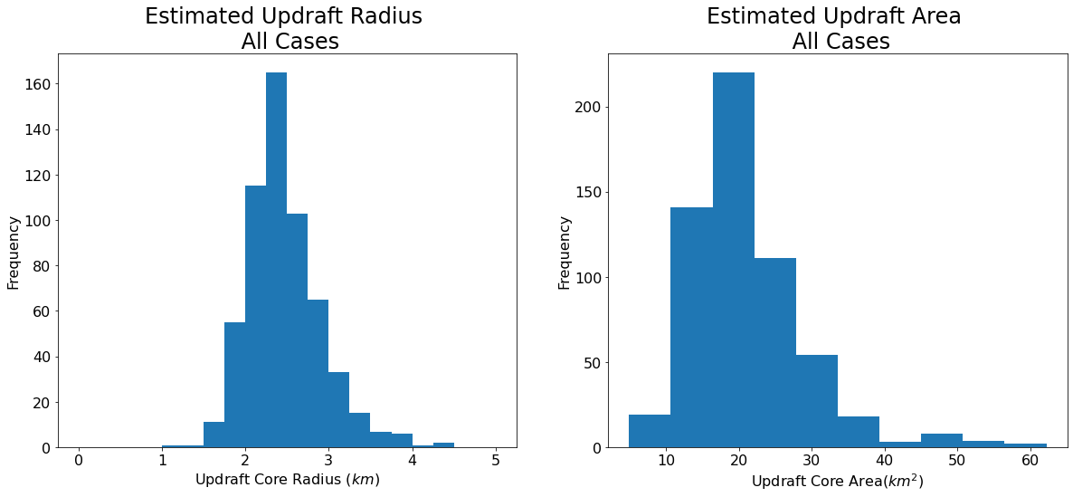
fig = plt.figure(figsize=(12,8))
plt.hist(max_depth, bins=otd_bins)

plt.title('OT Depth Distribution \n 14 November 2018 0000 - 0635 UTC', fontsize=24)

plt.xlabel('OT Depth (km)', fontsize=16)
plt.ylabel('Frequency', fontsize=16)

Text(0, 0.5, 'Frequency')

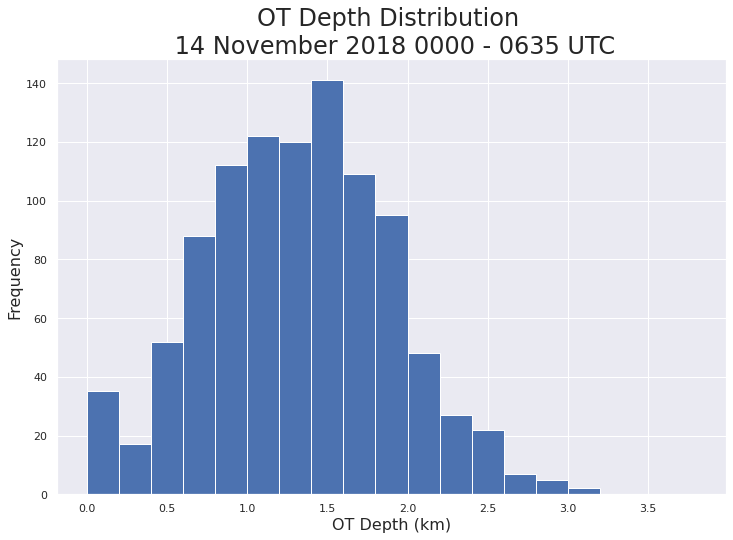
fig = plt.figure(figsize=(12,8))
plt.hist(duration, np.arange(2,20, 2))

plt.title('OT Depth Distribution \n 14 November 2018 0000 - 0635 UTC', fontsize=24)

plt.xlabel('OT Depth (km)', fontsize=16)
plt.ylabel('Frequency', fontsize=16)

Text(0, 0.5, 'Frequency')

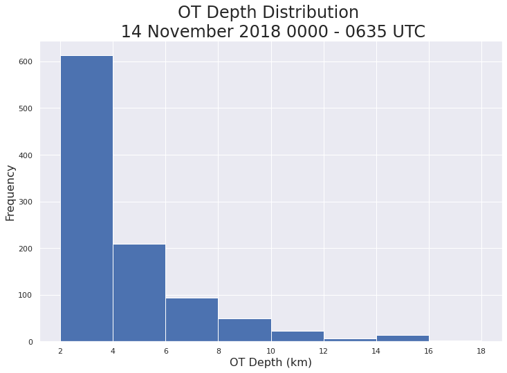
df = pd.DataFrame({'duration':duration,
              'max_ota':max_otarea,
              'mean_ota':mean_otarea})

df['round_ota'] = np.around(df.max_ota,-1)

df.boxplot('round_ota')

<AxesSubplot:>

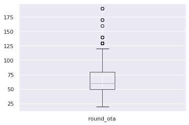
len(duration[np.where(duration > 2)])

939

import cartopy.feature as cfeature 
fig = plt.figure(figsize=(12,8))
ax = plt.subplot(111, projection=ccrs.PlateCarree())

ax.add_feature(cfeature.OCEAN)
ax.add_feature(cfeature.LAND)
ax.add_feature(cfeature.BORDERS, linestyle=':')

<cartopy.mpl.feature_artist.FeatureArtist at 0x2b80a64b0f60>

cells_grouped = trajectories_filtered.groupby('cell')



duration = cells_grouped.count().area_polygon.values
max_otarea = cells_grouped.max().area_polygon.values
mean_otarea = cells_grouped.mean().area_polygon.values

slope, intercept, r, p, stderr = scipy.stats.linregress(duration, max_otarea)

line = f'Regression line: y={intercept:.2f}+{slope:.2f}x, r={r:.2f}'

plt.figure(figsize=(10,8))
ax = plt.subplot(111)
ax.scatter(duration, max_otarea)
ax.plot(np.array(duration), intercept + slope * np.array(duration), label=line, color='black')

plt.ylabel('OT Area ($km^{2}$)', fontsize=12)
plt.xlabel('OT Duration (minutes)', fontsize=12)

plt.legend(loc='upper right', fontsize=12)

plt.title('OT Duration All OTs  \n 10 November, 12 November, 14 December 2018 UTC (Count = 5967)', fontsize=16)

llcrnr=[-33.206342, -65.906586]
urcrnr=[-30.255825, -62.630553]

# Set extent of maps created in the following cells:
axis_extent=[llcrnr[1],urcrnr[1],llcrnr[0],urcrnr[0]]    

# Plot map with all individual tracks:
import cartopy.crs as ccrs
fig_map,ax_map=plt.subplots(figsize=(15,15),subplot_kw={'projection': ccrs.PlateCarree()})

ax_map.coastlines()

ax_map.set_extent(axis_extent)

for ds in ds_list:
#    cm = ax.contourf(ds.x.values[::5], ds.y.values[::5], ds.values[::5,::5], levs, cmap='terrain', transform=ccrs.PlateCarree())
    cm = ax_map.imshow(ds.values, extent =[ds.x.min(),ds.x.max(),ds.y.min(),ds.y.max()], transform=ccrs.PlateCarree(), vmin=0, vmax=4000, cmap='terrain')

gl = ax_map.gridlines(crs=ccrs.PlateCarree(), draw_labels=True,
                  linewidth=2, color='gray', alpha=0.5, linestyle='--')

for name, group in cells_grouped:
#    print(group.x,group.y)
    plt.plot(group.lon,group.lat,"-o",markersize=1)

plt.colorbar(cm,label='Elevation (m)',shrink=0.6, pad=0.1)

ax_map.set_title('Overshooting top tracks\n All Cases')

Text(0.5, 1.0, 'Overshooting top tracks\n All Cases')

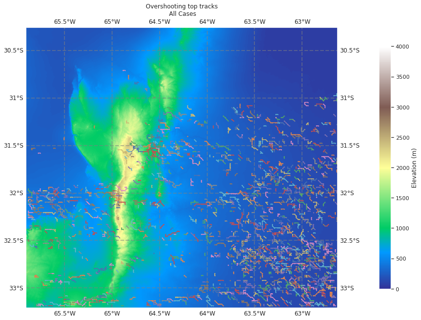
llcrnr=[-33.206342, -65.906586]
urcrnr=[-30.255825, -62.630553]

# Set extent of maps created in the following cells:
axis_extent=[llcrnr[1],urcrnr[1],llcrnr[0],urcrnr[0]]    

# Plot map with all individual tracks:
import cartopy.crs as ccrs
fig_map,ax_map=plt.subplots(figsize=(15,15),subplot_kw={'projection': ccrs.PlateCarree()})

ax_map.coastlines()

ax_map.set_extent(axis_extent)

for ds in ds_list:
#    cm = ax.contourf(ds.x.values[::5], ds.y.values[::5], ds.values[::5,::5], levs, cmap='terrain', transform=ccrs.PlateCarree())
    cm = ax_map.imshow(ds.values, extent =[ds.x.min(),ds.x.max(),ds.y.min(),ds.y.max()], transform=ccrs.PlateCarree(), vmin=0, vmax=4000, cmap='terrain')

gl = ax_map.gridlines(crs=ccrs.PlateCarree(), draw_labels=True,
                  linewidth=2, color='gray', alpha=0.5, linestyle='--')

for name, group in cells_grouped:
#    print(group.x,group.y)
    cm2 = plt.scatter(group.lon,group.lat,c=group.area_polygon,vmin=0.,vmax=200.,s=group.area_polygon,
                     facecolors='none',cmap='magma',linewidth=0.5)

plt.colorbar(cm,label='Elevation (m)',shrink=0.4, pad=0.0)
plt.colorbar(cm2,label='OT Area (km$^2$)',shrink=0.4, pad=0.1)



ax_map.set_title('Overshooting top tracks\n All Cases')

Text(0.5, 1.0, 'Overshooting top tracks\n All Cases')

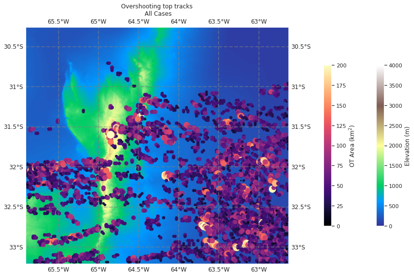
import seaborn as sns

sns.set()

plt.hist(duration)

(array([936., 317., 148.,  61.,  20.,  21.,  15.,   9.,   4.,   3.]),
 array([ 2. ,  3.8,  5.6,  7.4,  9.2, 11. , 12.8, 14.6, 16.4, 18.2, 20. ]),
 <BarContainer object of 10 artists>)

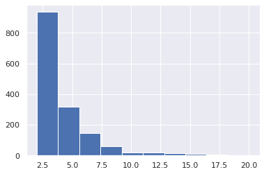
plt.figure(figsize=(10,8))
plt.hist(max_otarea, bins=np.arange(0, 300, 25))

(array([ 48., 524., 517., 279.,  85.,  43.,  21.,  13.,   2.,   2.,   0.]),
 array([  0,  25,  50,  75, 100, 125, 150, 175, 200, 225, 250, 275]),
 <BarContainer object of 11 artists>)

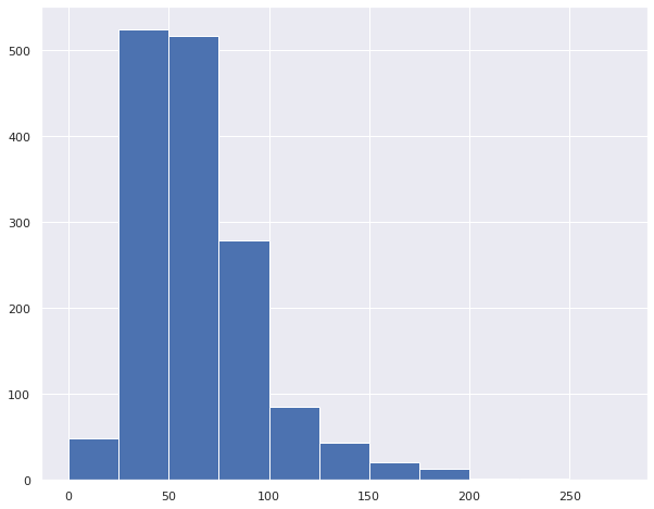
df_track= pd.read_csv('test.csv')

v_max=60.
stubs=2
order=1
extrapolate=1
memory=1
adaptive_stop=0.01
adaptive_step=0.99
subnetwork_size=100
method_linking= 'predict'
cell_number_start=1
dt = 60.
dxy = 2000.

search_range=dt*v_max

features_linking=deepcopy(df_track)

pred = tp.predict.NearestVelocityPredict(span=1)
trajectories_unfiltered = pred.link_df(features_linking, search_range=search_range, memory=memory,
                                 pos_columns=['x','y'],
                                 t_column='frame',
                                 neighbor_strategy='KDTree', link_strategy='auto',
                                 adaptive_step=adaptive_step,adaptive_stop=adaptive_stop
#                                 copy_features=False, diagnostics=False,
#                                 hash_size=None, box_size=None, verify_integrity=True,
#                                 retain_index=False
                                 )

trajectories_unfiltered['cell']=None
for i_particle,particle in enumerate(pd.Series.unique(trajectories_unfiltered['particle'])):
    cell=int(i_particle+cell_number_start)
    trajectories_unfiltered.loc[trajectories_unfiltered['particle']==particle,'cell']=cell
trajectories_unfiltered.drop(columns=['particle'],inplace=True)

trajectories_bycell=trajectories_unfiltered.groupby('cell')

num_stubs = 0

for cell,trajectories_cell in trajectories_bycell:
#    logging.debug("cell: "+str(cell))
#    logging.debug("feature: "+str(trajectories_cell['feature'].values))
#    logging.debug("trajectories_cell.shape[0]: "+ str(trajectories_cell.shape[0]))


    if trajectories_cell.shape[0] < stubs:
#        print("cell" + str(cell)+ "  is a stub ("+str(trajectories_cell.shape[0])+ "), setting cell number to Nan..")
        trajectories_unfiltered.loc[trajectories_unfiltered['cell']==cell,'cell']=np.nan
        num_stubs = num_stubs + 1

print('found this many stubs: {}'.format(num_stubs))

trajectories_filtered=trajectories_unfiltered.dropna()

Frame 15780: 1 trajectories present.
found this many stubs: 183

def test_prob(df, prob_thresh=.7, min_duration=2, max_prob_thresh=.7):
    test = df[df.prob > prob_thresh]
    
    cells_grouped = test.groupby('cell')
    
    max_vals = cells_grouped.max()
    duration = cells_grouped.count().area_polygon.values
    
    print(duration)
    max_prob_thresh = .7
    
    max_vals = max_vals[duration > min_duration]
    
    max_otarea = max_vals.area_polygon.values
    duration = duration[duration > min_duration]
    
    
    print(max_otarea)
    #mean_otarea = cells_grouped.mean()[duration > min_duration].area_polygon.values
    
    max_prob = max_vals.prob.values

    slope, intercept, r, p, stderr = scipy.stats.linregress(duration, max_otarea)

    line = f'Regression line: y={intercept:.2f}+{slope:.2f}x, r={r:.2f}'

    plt.figure(figsize=(10,8))
    ax = plt.subplot(111)
    s = ax.scatter(duration, max_otarea, s=50, c=max_prob, cmap='viridis_r')
    plt.colorbar(s, label='Max OT Probability')
    ax.plot(np.array(duration), intercept + slope * np.array(duration), label=line, color='black')

    plt.ylabel('OT Area ($km^{2}$)', fontsize=12)
    plt.xlabel('OT Duration (minutes)', fontsize=12)

    plt.legend(loc='upper right', fontsize=12)

    plt.title(f'OT Duration 14 December 2018 Prob Thresh: {prob_thresh} \n 1500 - 2359 UTC (Count = {len(max_prob)})', fontsize=16)
    
    plt.show()
    
    plt.close()

trajectories_filtered.groupby('cell')[trajectories_filtered.groupby('cell').count().area_polygon.values > 2]

---------------------------------------------------------------------------
KeyError                                  Traceback (most recent call last)
<ipython-input-183-716a39b269b3> in <module>
----> 1 trajectories_filtered.groupby('cell')[trajectories_filtered.groupby('cell').count().area_polygon.values > 2]

~/a/miniconda3/envs/xesmf_env/lib/python3.7/site-packages/pandas/core/groupby/generic.py in __getitem__(self, key)
   1648                 stacklevel=2,
   1649             )
-> 1650         return super().__getitem__(key)
   1651 
   1652     def _gotitem(self, key, ndim: int, subset=None):

~/a/miniconda3/envs/xesmf_env/lib/python3.7/site-packages/pandas/core/base.py in __getitem__(self, key)
    216             if len(self.obj.columns.intersection(key)) != len(key):
    217                 bad_keys = list(set(key).difference(self.obj.columns))
--> 218                 raise KeyError(f"Columns not found: {str(bad_keys)[1:-1]}")
    219             return self._gotitem(list(key), ndim=2)
    220 

KeyError: 'Columns not found: False, True'

duration = cells_grouped.count().area_polygon.values

test_prob(trajectories_filtered, .7, 2)

[ 5  2  2  2  4  2  4  5  3  2  4  3  7  5  2  2  3  2  4  9  8  2  3  4
  3  3  2  4  3  2  4  4  6  4  2  2  4  2  2  2  3  2  6  3  3  2  7  6
  4  4 11 12  2  9  3 11  2  7  7  3  2  2  3  3  2  4  3  2  2  3  5  6
  2 10  5  5  5  3  2  5  2  2  2  3  3  2  3  4  3  7  3  5  5  2  3  2
  7  6  5  2  3  4  2  2  2  8  3  5  6  7  4  2  7  2  2  6  4  2  2  6
  5  3  2  5  2  2  2  3  4  4  3  3  5  2  5  5  6  2  2  3  2  2  4  2
  3  3  3  7]
[ 53.04495093  74.95417576  37.22169946  36.22672045  50.61187799
  51.4434505   49.73851352  41.60106836  47.97494253  99.33966763
  37.05978449  62.73190927  37.34097974  98.73006191  54.95093377
  33.80301911  49.73551538  57.66338334  43.04843349  43.15796459
  61.58380279  47.34810358  56.40235019  35.98703749  71.76936767
  42.77964004  89.923258    26.88437875  42.40980711  53.30652372
  40.19559012  40.76121201  82.6356979   91.5173871   74.16442957
  27.1494529   91.64322272  49.21365175  55.84471987  63.73875001
  74.47165467  59.17907651  60.09637166  36.07194206  24.86860699
 153.22103771  79.01694039  52.0826308   50.69875666  80.15188931
  83.39018604  30.00008876 104.97386916  58.59652657  71.26936123
  34.65932185  58.80201834  61.68727596  67.29776296  62.69034573
  32.38741432  53.64826974  60.13650522  71.03616092  55.35387262
  76.03060243  86.04511828  47.63491399 143.8508524   32.68053654
  40.69231687  47.10273251  42.0614839   47.21424162  46.02778155
  55.44185684  39.57863298  31.61586932  72.69550589  45.24590701
  63.69588757  77.32296219  74.92618988  63.31117279  70.31960889
  80.26527122  37.88331172  36.65335523  33.02236218  49.23137937
  65.83118773  35.85408394  39.86269417  79.42777577  38.38252911
  68.43706303]

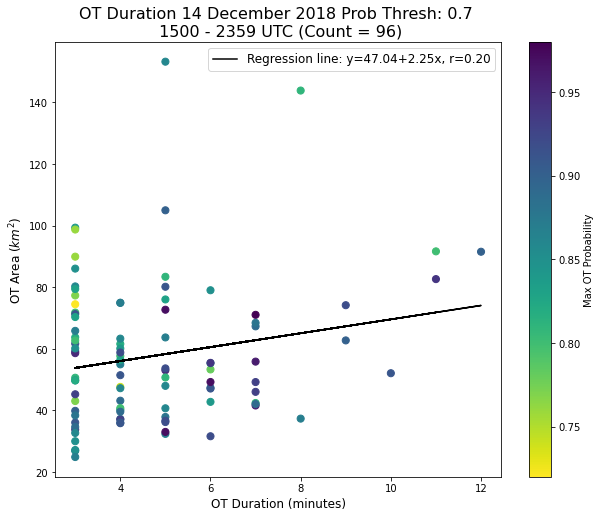
cells_grouped = test.groupby('cell')

duration = cells_grouped.count().area_polygon.values
max_otarea = cells_grouped.max().area_polygon.values
mean_otarea = cells_grouped.mean().area_polygon.values

slope, intercept, r, p, stderr = scipy.stats.linregress(duration, max_otarea)

line = f'Regression line: y={intercept:.2f}+{slope:.2f}x, r={r:.2f}'

plt.figure(figsize=(10,8))
ax = plt.subplot(111)
ax.scatter(duration, max_otarea)
ax.plot(np.array(duration), intercept + slope * np.array(duration), label=line, color='black')

plt.ylabel('OT Area ($km^{2}$)', fontsize=12)
plt.xlabel('OT Duration (minutes)', fontsize=12)

plt.legend(loc='upper right', fontsize=12)

plt.title('OT Duration 14 December 2018 \n 1500 - 2359 UTC (Count = 2353)', fontsize=16)

Text(0.5, 1.0, 'OT Duration 14 December 2018 \n 1500 - 2359 UTC (Count = 2353)')