Exploring a ZDR Offset Value
Contents
Exploring a ZDR Offset Value
import xarray as xr
import pyart
import numpy as np
import hvplot.xarray
import hvplot.pandas
import holoviews as hv
import warnings
import xcollection as xc
import glob
import matplotlib.pyplot as plt
import pandas as pd
import cartopy.crs as ccrs
from distributed import Client, LocalCluster
warnings.filterwarnings("ignore")
hv.extension('bokeh')


Read in the data
def create_dataset_from_sweep(radar, sweep=0, field=None):
"""
Creates an xarray.Dataset from sweeps
"""
# Grab the range
range = radar.range['data']
# Grab the elevation
elevation = radar.get_elevation(sweep)
# Grab the azimuth
azimuth = radar.get_azimuth(sweep)
# Grab the x, y, z values
x, y, z = radar.get_gate_x_y_z(sweep)
# Grab the lat, lon, and elevation
lat, lon, alt = radar.get_gate_lat_lon_alt(sweep)
# Add the fields
field_dict = {}
for field in list(radar.fields):
field_dict[field]=(["azimuth", "range"], radar.get_field(sweep, field))
ds = xr.Dataset(
data_vars=field_dict,
coords=dict(
x=(["azimuth", "range"], x),
y=(["azimuth", "range"], y),
z=(["azimuth", "range"], z),
lat=(["azimuth", "range"], lat),
lon=(["azimuth", "range"], lon),
alt=(["azimuth", "range"], alt),
azimuth=azimuth,
elevation=elevation,
sweep=np.array([sweep]),
range=range),
)
return ds.chunk()
def convert_to_xradar(radar):
"""
Converts from radar to xradar
"""
ds_list = []
sweeps = radar.sweep_number['data']
for sweep in sweeps:
ds_list.append(create_dataset_from_sweep(radar, sweep))
# Convert the numpy array to a list of strings
dict_keys = [x for x in list(sweeps.astype(str))]
# Zip the keys and datasets and turn into a dictionary
dict_of_dsets = dict(zip(dict_keys, ds_list))
return xc.Collection(dict_of_dsets)
List files available
We grab the files from the following directory, after ordering from the data portal and unzipping the archive
We use 6 degree elevation scans from the CSU X-Band Radar
radar_files = sorted(glob.glob('../../data/x-band/ppi/*6_PPI.nc'))
Spin up a Dask Cluster
cluster = LocalCluster()
client = Client(cluster)
client
Client
Client-5d56539a-ac5a-11ec-b946-acde48001122
| Connection method: Cluster object | Cluster type: distributed.LocalCluster |
| Dashboard: http://127.0.0.1:57028/status |
Cluster Info
LocalCluster
32bb9ac9
| Dashboard: http://127.0.0.1:57028/status | Workers: 4 |
| Total threads: 12 | Total memory: 16.00 GiB |
| Status: running | Using processes: True |
Scheduler Info
Scheduler
Scheduler-ac7f2c95-5a81-4ae6-87cb-56f6514dcb06
| Comm: tcp://127.0.0.1:57029 | Workers: 4 |
| Dashboard: http://127.0.0.1:57028/status | Total threads: 12 |
| Started: Just now | Total memory: 16.00 GiB |
Workers
Worker: 0
| Comm: tcp://127.0.0.1:57042 | Total threads: 3 |
| Dashboard: http://127.0.0.1:57049/status | Memory: 4.00 GiB |
| Nanny: tcp://127.0.0.1:57034 | |
| Local directory: /Users/mgrover/git_repos/SAILS-radar-analysis/notebooks/march-14-2022/dask-worker-space/worker-dayqk35x | |
Worker: 1
| Comm: tcp://127.0.0.1:57045 | Total threads: 3 |
| Dashboard: http://127.0.0.1:57048/status | Memory: 4.00 GiB |
| Nanny: tcp://127.0.0.1:57035 | |
| Local directory: /Users/mgrover/git_repos/SAILS-radar-analysis/notebooks/march-14-2022/dask-worker-space/worker-iu_qokz5 | |
Worker: 2
| Comm: tcp://127.0.0.1:57043 | Total threads: 3 |
| Dashboard: http://127.0.0.1:57046/status | Memory: 4.00 GiB |
| Nanny: tcp://127.0.0.1:57032 | |
| Local directory: /Users/mgrover/git_repos/SAILS-radar-analysis/notebooks/march-14-2022/dask-worker-space/worker-_jwg59jp | |
Worker: 3
| Comm: tcp://127.0.0.1:57044 | Total threads: 3 |
| Dashboard: http://127.0.0.1:57047/status | Memory: 4.00 GiB |
| Nanny: tcp://127.0.0.1:57033 | |
| Local directory: /Users/mgrover/git_repos/SAILS-radar-analysis/notebooks/march-14-2022/dask-worker-space/worker-gqcillks | |
Loop through and read in the data
ds = convert_to_xradar(pyart.io.read(radar_files[0]))['0']
Clean the Data
We will drop a couple of coordinates, and make sure that we don’t include the fill values (which are large negative numbers)
ds = ds.drop(['elevation', 'sweep'])
Set which fields to plot in the interactive plot
fields = ['DBZ', 'VEL', 'ZDR']
for field in fields:
da = ds[field]
ds[field] = ds[field].where(da > -999)
ds.compute().hvplot.quadmesh(x='lon',
y='lat',
ylabel='Latitude',
xlabel='Longitude',
z=['DBZ', 'VEL', 'ZDR'],
rasterize=True,
width=600,
height=400,
geo=True,
alpha=0.1,
selection_color={'NaN': (0, 0, 0, 0)},
#projection=ccrs.PlateCarree(),
cmap='pyart_Carbone42',
features={'rivers':'110m'},
tiles='StamenTerrainRetina').opts("Image", alpha=0.8)
Apply a first pass filter
We apply a filter for:
cross-corrlation coefficient (
RHOHV) > 0.95non-coherent power (
NCP) > 0.5
ds_filtered = ds.where((ds.RHOHV > 0.95) & (ds.NCP > 0.5))
Plot the Filtered Dataset
Let’s take a look at the filtered data, using a plotting template function.
def plot_field(field='DBZ',
color_bounds=(-20, 40),
cmap='pyart_Carbone42',
ds_to_plot=ds_filtered):
plot = ds_to_plot[field].compute().hvplot.quadmesh(x='lon',
y='lat',
ylabel='Latitude',
xlabel='Longitude',
clim=color_bounds,
rasterize=True,
xlim=(-107.1, -106.8),
ylim=(38.8, 39.1),
width=600,
height=400,
geo=True,
alpha=0.1,
projection=ccrs.PlateCarree(),
cmap=cmap,
title=field,
features={'rivers':'110m'},
tiles='StamenTerrainRetina').opts("Image",
alpha=0.8)
return plot
ref_plot = plot_field('DBZ', (-20, 40))
vel_plot = plot_field('VEL', (-15, 15), cmap='pyart_balance')
zdr_plot = plot_field('ZDR', (-2, 1))
(ref_plot + vel_plot + zdr_plot).cols(1)
Investigate Histograms
Reflectivity
dbz_hist = ds_filtered.DBZ.hvplot.hist(bins=np.arange(-40, 40, 1), title='DBZ Values')
dbz_hist
NCP
ncp_hist = ds_filtered.NCP.hvplot.hist(bins=np.arange(.7, 1.01, 0.01), title='NCP Values')
ncp_hist
ZDR
zdr_hist = ds_filtered.ZDR.hvplot.hist(bins=np.arange(-3, 1.1, .1), title='ZDR Values')
zdr_hist
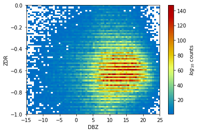
Plot a 2D histogram using matplotlib
bins = np.linspace(-15, 25, 71)
zdr_bins = np.linspace(-1, 0, 71)
hist = np.histogram2d(ds_filtered.ZDR.values.flatten(),
ds_filtered.DBZ.values.flatten(),
bins=70,
range=((-1, 0), (-15, 25)))[0]
hist = np.ma.masked_where(hist == 0, hist)
# Create a 1-1 comparison
#x, y = np.meshgrid((-5, 1),(-6, 20))
c = plt.pcolormesh(bins,
zdr_bins,
hist,
cmap='pyart_HomeyerRainbow')
# Add a colorbar and labels
plt.colorbar(c, label='$log_{10}$ counts')
plt.xlabel('DBZ')
plt.ylabel('ZDR')
plt.show()
Plot a 2D Hexbin Visualization
zdr = ds_filtered.ZDR.values.flatten()
dbz = ds_filtered.DBZ.values.flatten()
df = pd.DataFrame({'ZDR':zdr,
'DBZ':dbz})
min_zdr = -2
max_zdr = 1
df_range = df[(df.ZDR >= min_zdr) &
(df.ZDR < max_zdr)]
df_range.hvplot.hexbin('DBZ',
'ZDR',
rasterize=True,
cmap='pyart_HomeyerRainbow',
logz=True,
)